Integrating R and C
R can be interfaced with both C and C++, coming with a significant speed up in computation time and efficiency. R has an inbuilt system for calling C with the .Call function, and RCpp can be used to integrate more easily with C++, enabling the use of pre-existing functions similar to those in base R. This portfolio will detail how this integration between R and C is possible effectively through the use of examples in a statistical sense.
Adaptive Kernel Regression Smoothing
In the situation where we have some data which can not fit into a conventional linear model, we can employ the use of kernel smoothing to fit a more flexible model. More specifically, suppose the data has been generated from the following model \[ y_i = \sin(\alpha \pi x^3) + \epsilon_i, \qquad \text{ with } \qquad \epsilon_i \sim N(0, \sigma^2), \] where \(x\) is a uniformly random sample, and \(\alpha\) and \(\sigma\) are fixed parameters. This simulated data can be generated in R with parameter values \(\alpha = 4\) and \(\sigma=0.2\), for \(i=1,\dots, n\):
set.seed(998)
n = 200
x = runif(n)
y = sin(4*pi*x^3) + rnorm(n, 0, 0.2)
plot(x, y, pch = 20)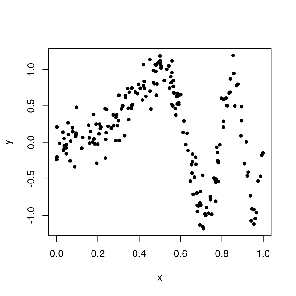 From the plot it is clear that the data are non-linear, so a simple linear model would not be suitable. A kernel regression smoother can be used to estimate the conditional expectation \(\mu(x) = \mathbb{E}(y|x)\) more flexibly using
\[
\hat{\mu}(x) = \frac{\sum^n_{i=1}\kappa_\lambda (x, x_i)y_i}{\sum^n_{i=1}\kappa_\lambda(x, x_i)},
\]
where \(\kappa\) is a kernel with bandwidth \(\lambda > 0\). This kernel regression can be written in R as well as C, so it provides opportunity for comparison between the two languages.
From the plot it is clear that the data are non-linear, so a simple linear model would not be suitable. A kernel regression smoother can be used to estimate the conditional expectation \(\mu(x) = \mathbb{E}(y|x)\) more flexibly using
\[
\hat{\mu}(x) = \frac{\sum^n_{i=1}\kappa_\lambda (x, x_i)y_i}{\sum^n_{i=1}\kappa_\lambda(x, x_i)},
\]
where \(\kappa\) is a kernel with bandwidth \(\lambda > 0\). This kernel regression can be written in R as well as C, so it provides opportunity for comparison between the two languages.
Writing a function in C
We can write a C function to implement a Gaussian kernel with variance \(\lambda^2\), shown below.
#include <R.h>
#include <Rinternals.h>
#include <Rmath.h>

SEXP meanKRS(SEXP y, SEXP x, SEXP x0, SEXP lambda)
{

  int n, n0;
  double lambda0;
  double *outy, *x00, *xy, *y0;

  n0 = length(x0);

  x = PROTECT(coerceVector(x, REALSXP));
  y = PROTECT(coerceVector(y, REALSXP));
  SEXP out = PROTECT(allocVector(REALSXP, n0));

  n = length(x);

  outy = REAL(out);
  lambda0 = REAL(lambda)[0];
  x00 = REAL(x0);
  xy = REAL(x);
  y0 = REAL(y);

  for(int i=0; i<n0; i++)
  {
    double num = 0, den = 0;
    for(int j=0; j<n; j++)
    {
      num += dnorm(xy[j], x00[i], lambda0, 0)*y0[j];
      den += dnorm(xy[j], x00[i], lambda0, 0);
    }
    outy[i] = num/den;
  }

  UNPROTECT(3);

  return out;
}
This is a large, and quite complicated function to what would normally be implemented in R. The main reason for the length of the function is due to the amount of declarations that have to be made in C. At the start, all integers and doubles are declared, with a * signifying that these are pointers, which instead point to a location in memory rather than being a variable themselves. x, y and out are all defined as vectors; either defining the inputs or allocating a new vector, with PROTECT signifying that these locations in memory are protected. Then the pointers are set up with the REAL function deciding where to point, and the [0] index meaning to take the value of where is being pointed to instead of setting up a pointer.
After this, the actual kernel smoothing is calculated within two for loops, as there is no global definition for sum in C. The numerator num and denominator den are defined on each iteration of the outer loop, and they are added to themselves in the inner loop. Once the inner loop iterations are complete, the value of out is assigned as the division of these two (which is pointed to by outy). Finally, the protected vectors are unprotected, to free up memory.
The headers at the beginning of the file, written as #include <header.h> allow the inclusion of certain pre-written functions that make writing C code simpler. Using the R, Rinternals and Rmath were not all necessary, however Rmath provided the dnorm function that was necessary for the Gaussian kernel.
Also note that the use of a double for loop is not inefficient in C as it would be in R, so there is no significant slowdown coming from nested loops. Now the function is written, it can be saved into the current working directory and loaded into R.
system("R CMD SHLIB meanKRS.c")
dyn.load("meanKRS.so")
A wrapper function can be set up to clean up code, i.e. an R function can be made which explicitly calls the C function with the same arguments. After this, we can plot the results to see how the smoothing looks with an arbitrary value of \(\lambda^2 = 0.02\).
meanKRS = function(y, x, x0, lambda) .Call("meanKRS", y, x, x0, lambda)
plot(x, y, pch = 20)
lines(seq(0, 1, len=1000), meanKRS(y, x, seq(0,1,len=1000), lambda = 0.02), col="blue", lwd=2)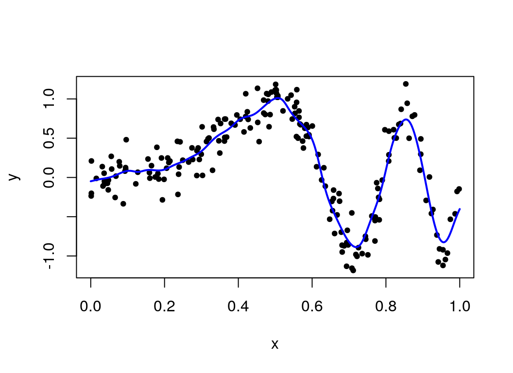
So this kernel smoothing approach has provided a nice fit to the simulated data, and appears to be going through the centre of the points across the plot.
To compare the computational efficiency, we can compare this C function with a simpler function written in R, called meanKRS_R (function not shown here for brevity, the R function performs the same operation whilst making use of R’s sum function instead of having a loop).
all.equal(meanKRS_R(y,x,seq(0,1,len=1000),0.06), meanKRS(y,x,seq(0,1,len=1000),0.06))## [1] TRUESo the values are exactly the same, and the function is accurate. How much quicker is it? We can use microbenchmark to display summary statistics of timing both functions 100 times.
library(microbenchmark)
microbenchmark(C_KRS = meanKRS(y,x,seq(0,1,len=1000),0.06),
               R_KRS = meanKRS_R(y,x,seq(0,1,len=1000),0.06), times = 100)
## Unit: milliseconds
## expr min lq mean median uq max neval
## C_KRS 14.32545 16.17882 16.36242 16.27690 16.42271 20.37999 100
## R_KRS 30.25504 32.08685 33.45924 32.42864 34.38512 43.47946 100So the C code is significantly faster, as expected, by about a factor of two.
Implementing cross-validation
The value of \(\lambda\) used here was chosen arbitrarily, but in practice it is common to use \(k\)-fold cross-validation to choose a more optimal value of \(\lambda\). We can implement a cross-validation routine in C. Implementing a function within a function is difficult in C, but it is relatively straightforward in Rcpp. This example goes through the use of Rcpp to implement cross-validation.
Rcpp is a package in R which provides tools to implement C++ code in R. It works in a similar way to how the .Call interface works for C code, but with a more accessible interface. Firstly, we create a file in the working directory called KRS_cv.cpp, where the Rcpp functions will be stored. This file contains a few functions, the first of which being the meanKRS function re-written for Rcpp.
// [[Rcpp::export(name = "meanKRS")]]
NumericVector meanKRS_I(const NumericVector y, const NumericVector x,
                        const NumericVector x0, const double lambda)
{
  int n, n0;
  n0 = x0.size();
  n = x.size();
  NumericVector out(n0);
  for(int i=0; i<n0; i++)
  {
    double num = 0, den = 0;
    NumericVector dval = dnorm(x, x0[i], lambda, 1);
    double max_dval = max(dval);
    for(int j=0; j<n; j++)
    {
      num = num + exp(dval[j]-max_dval)*y[j];
      den = den + exp(dval[j]-max_dval);
    }
    out[i] = num/den;
  }
  return out;
}
The cross-validation function cvKRS is written as:
// [[Rcpp::export(name = "cvKRS")]]
NumericVector cvKRS_I(const NumericVector y, const NumericVector x,
                      const int k, const NumericVector lambdas)
{
  // declare variables and vectors
  int n = y.size();
  NumericVector mse_lambda(lambdas.size());
  NumericVector out(1);
  NumericVector sorted_x(n);
  NumericVector sorted_y(n);

  // sort x and y according to the order of x
  IntegerVector order_x = stl_order(x);
  for(int kk=0; kk < n; kk++)
  {
    int ind = order_x[kk]-1;
    sorted_y[kk] = y[ind];
    sorted_x[kk] = x[ind];
  }

  // set up indices to cross-validate for
  IntegerVector idxs = seq_len(k);
  IntegerVector all_idxs = rep_each(idxs, n/k);

  // different lambdas
  for(int jj = 0; jj < lambdas.size(); jj++)
  {
    double lambda = lambdas[jj];
    NumericVector mse(k);

    // cross-validation loop
    for(int ii=1; ii <= k; ii++)
    {
      const LogicalVector kvals = all_idxs != ii;

      NumericVector y_t = clone(sorted_y);
      NumericVector x_t = clone(sorted_x);
      NumericVector y_cross = y_t[kvals];
      NumericVector x_cross = x_t[kvals];
      NumericVector fit = meanKRS_I(y_cross, x_cross, sorted_x, lambda);

      // calculate mean squared error
      NumericVector error = pow((fit[!kvals] - sorted_y[!kvals]), 2);
      mse[ii-1] = mean(error);
    }

    // average mean squared error for each value of lambda
    mse_lambda[jj] = mean(mse);
  }

  // output lambda which gave the smallest mean squared error
  int best_pos = which_min(mse_lambda);
  out[0] = lambdas[best_pos];

  return out;
}
Comments within the function (succeeding a //) give explanation of each section of the function. This function also calls the other function meanKRS by using meanKRS_I. The function was defined as meanKRS_I in the .cpp file, but when exported into R it is defined as meanKRS, based on the comment preceeding the function definition. Both functions were defined within the same file, and so can call one another, provided the function being called is defined first. There is a function used within cvKRS that is not part of base Rcpp functionality: stl_order. This does the same thing as order in base R, but needed to be defined separately.
Now that the function is defined, we can call it within R by first loading the Rcpp library and then using the sourceCpp function to source the C++ file, located in the same working directory.
library(Rcpp)
sourceCpp("KRS_cv.cpp")
This is the stage where we would get compilation errors, if there were any. Now we can run the function over a series of \(\lambda\) values and plot the kernel regression over the simulated data for the optimal \(\lambda\) selected by cross-validation.
lambda_seq = exp(seq(log(1e-6),log(100),len=50))
best_lambda = cvKRS(y, x, k = 20, lambdas = lambda_seq)
plot(x, y, pch = 20)
lines(seq(0, 1, len=1000), meanKRS(y, x, seq(0,1,len=1000), best_lambda),
      col="deeppink", lwd=2)
To compare computational efficiency, we can benchmark speeds against a function written in R (not shown here).
microbenchmark(cvKRS(y, x, k = 20, lambdas = lambda_seq),
               cvKRS_R(y, x, k = 20, lambdas = lambda_seq),
               times = 5)
## Unit: seconds
## expr min lq mean
## cvKRS(y, x, k = 20, lambdas = lambda_seq) 2.289333 2.293236 2.660317
## cvKRS_R(y, x, k = 20, lambdas = lambda_seq) 6.390262 6.629278 7.100683
## median uq max neval
## 2.380029 3.141275 3.197711 5
## 7.481269 7.486666 7.515939 5So this further exemplifies the significant speed increase that comes with writing in C, or Rcpp. In fact, this function had an average of three times the speed of that of the R function, against the two times speed up the previous function had. This is likely due to using two functions written in C++ (as cross validation calls the original kernel regression function).
This has improved the fit, but no single value of \(\lambda\) leads to a satisfactory fit, due to the first half of the function (for \(x < 0.5\)) wanting a smooth \(\mu(x)\) as it is quite linear, and the second half wanting a less smooth one, as it is more ‘wiggly’. We can let the smoothness depend on \(x\) by constructing \(\lambda(x)\), which will improve the fit. This method is based around modelling the residuals and varying \(\lambda\) more when the residuals are larger. Thus in practice \(\lambda(x)\) is a sequence of values instead of a single value. Below are the contents of the file that contains the functions to implement this written in Rcpp.
#include <Rcpp.h>
using namespace Rcpp;

NumericVector fitKRS(const NumericVector x, const NumericVector x0,
                     const double lambda, const NumericVector y,
                     const NumericVector lambda_vec)
{
  NumericVector copy_y = clone(y);
  int n = x.size();
  int n0 = x0.size();
  NumericVector out(n0);
  for(int ii=0; ii<n0; ii++)
  {
    NumericVector dval = dnorm(x, x0[ii], lambda*lambda_vec[ii], 1);
    double max_dval = max(dval);
    double num=0, den=0;
    for(int jj=0; jj<n; jj++)
    {
      num = num + exp(dval[jj] - max_dval)*copy_y[jj];
      den = den + exp(dval[jj] - max_dval);
    }
    out[ii] = num/den;
  }
  return out;
}

// [[Rcpp::export(name = "mean_var_KRS")]]
NumericVector mean_var_KRS_I(const NumericVector y, const NumericVector x,
                             const NumericVector x0, const double lambda)
{
  int n = x.size();
  int n0 = x0.size();
  NumericVector res(n);
  NumericVector lambda_1sn(n, 1.0);
  NumericVector lambda_1sn0(n0, 1.0);
  NumericVector mu = fitKRS(x, x, lambda, y, lambda_1sn);
  NumericVector resAbs = abs(y - mu);
  NumericVector madHat = fitKRS(x, x0, lambda, resAbs, lambda_1sn0);
  NumericVector w = 1 / madHat;
  w = w / mean(w);
  NumericVector out = fitKRS(x, x0, lambda, y, w);

  return out;
}
The first function, fitKRS was used to save space, since the same operation is performed multiple times with different parameters. Different weightings w get added to the vector of \(\lambda\) values in the final stage, resulting in the varied \(\lambda(x)\) parameter. We can plot this to show this change, using the initial value of \(\lambda\) selected by cross-validation earlier.
sourceCpp("meanvarKRS.cpp")
varied_mu = mean_var_KRS(y = y, x = x, x0 = seq(0,1,len=1000), lambda = best_lambda)
plot(x, y, pch=20)
lines(seq(0, 1, len=1000), varied_mu, col = "darkgoldenrod", lwd=2)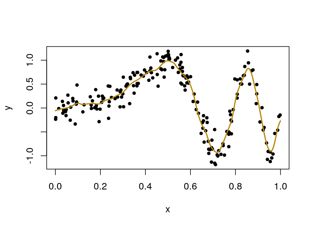 This looks like a good fit, and the function is working as intended. How well does the speed of the function written in Rcpp compare to one written in R?
microbenchmark(C = mean_var_KRS(y = y, x = x, x0 = seq(0,1,len=1000),
                                lambda = best_lambda),
               R = mean_var_KRS_R(y = y, x = x, x0 = seq(0,1,len=1000),
                                  lam = best_lambda), times = 500)
## Unit: milliseconds
## expr min lq mean median uq max neval
## C 25.56793 35.80579 41.67632 39.84551 45.09670 84.63745 500
## R 35.03011 54.59121 64.87276 61.94020 70.77707 122.68250 500This has an expected speed up again. And to make sure both functions are outputting the same thing, we can use all.equal again:
all.equal(mean_var_KRS(y = y, x = x, x0 = seq(0,1,len=1000),
                              lambda = best_lambda),
          mean_var_KRS_R(y = y, x = x, x0 = seq(0,1,len=1000),
                             lam = best_lambda))
## [1] TRUECross Validation Again
The value of \(\lambda\) used for fitting this local regression is that picked from cross-validation where \(\lambda\) does not vary with \(x\), in the previous section. To improve this fit further, we can use cross-validation again, but fitting the model with the new mean_var_KRS function on each iteration instead of the basic kernel regression. The function is written in Rcpp below.
// [[Rcpp::export(name = "mean_var_cv_KRS")]]
NumericVector mean_var_cv_KRS_I(const NumericVector y, const NumericVector x,
                      const int k, const NumericVector lambdas)
{
  int n = y.size();
  NumericVector mse_lambda(lambdas.size());
  NumericVector out(1);
  NumericVector sorted_x(n);
  IntegerVector order_x = stl_order(x);
  NumericVector test;
  NumericVector sorted_y(n);
  for(int kk=0; kk < n; kk++)
  {
    int ind = order_x[kk]-1;
    sorted_y[kk] = y[ind];
    sorted_x[kk] = x[ind];
  }
  IntegerVector idxs = seq_len(k);
  IntegerVector all_idxs = rep_each(idxs, n/k);

  for(int jj = 0; jj < lambdas.size(); jj++)
  {
    double lambda = lambdas[jj];
    NumericVector mse(k);
    for(int ii=1; ii <= k; ii++)
    {
      const LogicalVector kvals = all_idxs != ii;
      NumericVector y_t = clone(sorted_y);
      NumericVector x_t = clone(sorted_x);
      NumericVector y_cross = y_t[kvals];
      NumericVector x_cross = x_t[kvals];
      NumericVector fit = mean_var_KRS_I(y_cross, x_cross, sorted_x, lambda);
      NumericVector error = pow((fit[!kvals] - sorted_y[!kvals]), 2);
      mse[ii-1] = mean(error);
    }
    mse_lambda[jj] = mean(mse);
  }
  int best_pos = which_min(mse_lambda);
  out[0] = lambdas[best_pos];

  return out;
}
This functions is very similar to the cross-validation function implemented earlier. It loops over different values of \(\lambda\), but instead uses these as a starting point to fit a series of points using \(\lambda(x)\). The error is calculated against the cross-validated points and the starting \(\lambda\) that results in the smallest error is returned. Now we can call this in R, and re-run the mean_var_KRS function with the newly selected \(\lambda\) and see how it compares.
sourceCpp("meanvarcvKRS.cpp")
cv_best_lambda = mean_var_cv_KRS(y, x, k=20, exp(seq(log(0.01), log(1), len=50)))
cv_varied_mu = mean_var_KRS(y = y, x = x, x0 = seq(0,1,len=1000), lambda = cv_best_lambda)
plot(x, y, pch=20)
lines(seq(0, 1, len=1000), cv_varied_mu, col = "darkorchid", lwd=2)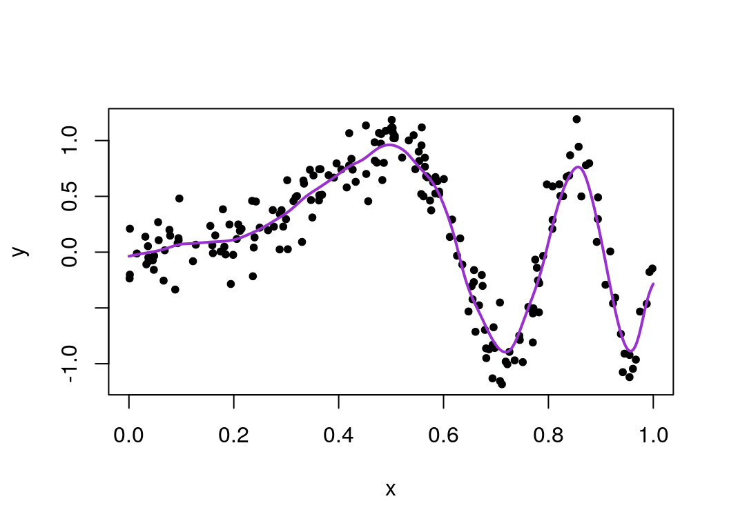 This looks a lot smoother for lower values of \(x\) than before, which looks like a better fit overall!
A way to improve this model might involve a local regression approach, which would be fitting parameter values at different (possibly uniform) intervals across the data set. Local regression will be covered in the next section.