Prostate Cancer Data

To give an example of using a least squares solver, we can use prostate cancer data given by the lasso2 package. If this package is not installed, we can use

install.packages("lasso2")

to install it. Once this package is installed, we obtain the dataset by running the commands

library(lasso2)
data(Prostate)

which gives us the dataset in our R environment. We start by inspecting the dataset, which can be done with

head(Prostate)

##       lcavol  lweight age      lbph svi       lcp gleason pgg45       lpsa
## 1 -0.5798185 2.769459  50 -1.386294   0 -1.386294       6     0 -0.4307829
## 2 -0.9942523 3.319626  58 -1.386294   0 -1.386294       6     0 -0.1625189
## 3 -0.5108256 2.691243  74 -1.386294   0 -1.386294       7    20 -0.1625189
## 4 -1.2039728 3.282789  58 -1.386294   0 -1.386294       6     0 -0.1625189
## 5  0.7514161 3.432373  62 -1.386294   0 -1.386294       6     0  0.3715636
## 6 -1.0498221 3.228826  50 -1.386294   0 -1.386294       6     0  0.7654678

Here we can see all the different elements of the dataset, which are:

• lcavol: The log of the cancer volume
  
• lweight: The log of the prostate weight
  
• age: The individual’s age
  
• lbph: The log of the benign prostatic hyperplasia amount
  
• svi: The seminal vesicle invasion
  
• lcp: The log of the capsular penetration
  
• gleason: The Gleason score
  
• pgg45: The percentage of the Gleason scores that are 4 or 5
  
• lpsa: The log of the prostate specific antigen

We don’t need to understand what all of these are, but we need to define what the inputs and outputs are. We are interested in the cancer volume, so setting \(\boldsymbol{y}\) as lcavol and \(\boldsymbol{x}\) as the other variables would measure how these other variables affect cancer volume. We can set this by running

y = as.vector(Prostate$lcavol)
X = model.matrix(~., data=Prostate)

which gives us our inputs and outputs. We are selecting the \(X\) matrix going from 2 to dim(Prostate)[2], which means that we are selecting the Prostate dataset from the second column to the last one (not including the response as a predictor). If our output variable was in a different column, we would exclude a different column using similar methods.

Now that we have set up the inputs and outputs, we can use the solution \[ \boldsymbol{w}_{LS} = (\boldsymbol{XX}^T)^{-1}\boldsymbol{Xy}^T. \] to find the coefficients \(\boldsymbol{w_{LS}}\). Converting this equation into R is done with the command:

wLS = solve(t(X) %*% X) %*% t(X) %*% y

The t(X) function simply takes the transpose of the matrix. The %*% function is just selecting matrix multiplication, as opposed to using * which would be element-wise multiplication. The solve function finds the inverse of a matrix, so solve(X) would give \(X^{-1}\). Now we have our coefficients

wLS

##                      [,1]
## (Intercept) -2.997602e-14
## lcavol       1.000000e+00
## lweight     -1.214306e-14
## age         -1.049508e-16
## lbph         6.045511e-16
## svi         -2.952673e-14
## lcp          4.538037e-15
## gleason      1.547373e-15
## pgg45       -2.255141e-17
## lpsa         1.706968e-15

which can be used to get the predicting function \(f(\boldsymbol{x};\boldsymbol{w})\) for these given inputs.

f = X %*% wLS

We can see how close the predicted output is to the actual output with a plot. If our predictions are accurate, then they will be close to the actual output, and lie on a diagonal line. We can plot these two values against each other using the command:

plot(f,y,xlab = "Predicted Values", ylab = "Actual Values", main = "Log of Cancer Volume")
abline(0,1)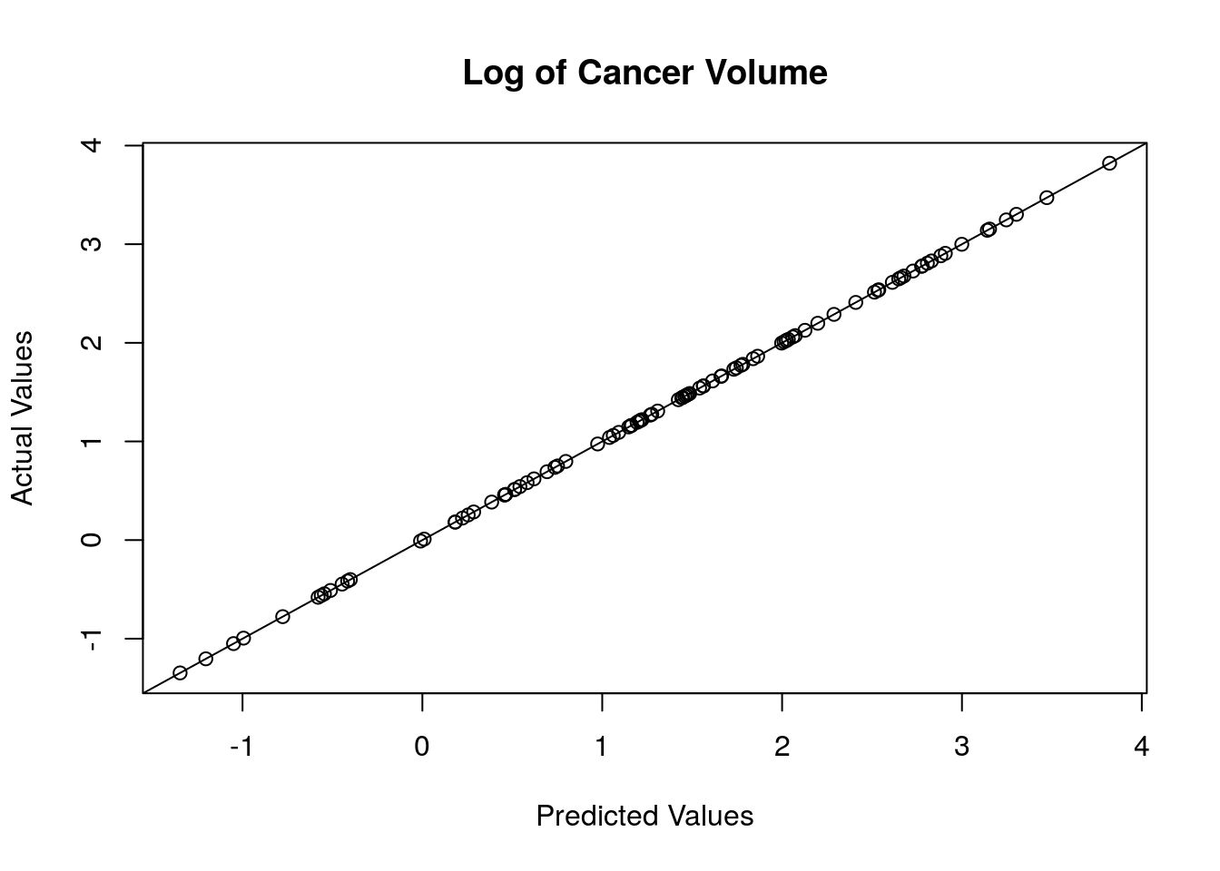

These match up almost perfectly, so our predictions are accurate.

Cross-validation

Cross-validation is a general purpose method for evaluating the method of the predicting function \(f(\boldsymbol{x};\boldsymbol{w})\). This is done by leaving \(n\) points out of the dataset, fitting the coefficients to the remaining dataset, then using the new coefficients to create a new predicting function which can predict the data point that was missed out. The difference between this predicted point and the actual observed point can be used as a metric to judge the accuracy of the predicting function.

In more technical terms, we split the dataset \(D\) into \(k\) distinct subsets \(D_1, \dots, D_k\), and fit \(f_{-i}(\boldsymbol{x}_{-i};\boldsymbol{w})\) for each dataset and for \(i=0,\dots k\). We then take the squared error between \(y_i\) and \(f(\boldsymbol{x}_{i};\boldsymbol{w})\), and average across all subsets, i.e. \[ \frac{1}{k+1} \sum^k_{i=1} \left[ f(\boldsymbol{x}_{i};\boldsymbol{w}) - y_i \right]^2 \] To do this in R, we can set up a loop that will create a new data subset on each iteration, carry out the same procedure as detailed before to obtain the coefficients and the predicting function, measure the error and repeat \(k\) times. This is done with:

N = length(y)
error = numeric(N)
for(i in 1:N){
  Xmini = X[-i,]
  ymini = y[-i]
  wLSmini = solve(t(Xmini) %*% Xmini) %*% t(Xmini) %*% ymini
  fout = X[i,] %*% wLSmini
  error[i] = (fout - y[i])^2
}

Using the indexing of X[-i,] will subset X to all rows except the \(i\)-th one. With this reduced data set, as well as only using the \(y_{-i}\) inputs, we estimate the coefficients at each iteration and then use that to calculate the squared error, which is saved in the error array. To find the overall error, we just take the mean of this array.

mean(error)

## [1] 3.701126e-27

Removing Features

We can use this overall squared error as a reference point, because it can be compared against the same score when removing certain inputs (columns of X) to see if the prediction function is more accurate without some of these included. We can do this by setting up another loop that loops over the number of inputs, and performing the same methods as before to calculate the averages. This is done with:

D = dim(X)[2]
error_all = numeric(D-1)
for(d in 2:D){
  Xd = X[,-d] 
  error_d = numeric(N)
  for(i in 1:(dim(X)[1])){
    Xmini = Xd[-i,]
    ymini = y[-i]
    wLSmini = solve(t(Xmini) %*% Xmini) %*% t(Xmini) %*% ymini
    fout = Xd[i,] %*% wLSmini
    error_d[i] = (fout - y[i])^2
  }
  error_all[d-1] = mean(error_d)
} 

So this starts with setting the array error_all to the length of the number of inputs. Then there is a loop which iterates over the number of inputs (excluding the first column, which corresponds to the intercept), and removes a column from X, renaming it Xd. Another array is set up, called error_d, which is equivalent to the error array from the previous section. The nested loop performs the same operation as the cross-validation before. We can inspect this array, and compare it against the previous cross-validation error:

error_all

## [1] 5.351267e-01 2.736666e-27 3.654340e-27 3.473490e-27 3.802165e-27
## [6] 4.893871e-27 9.457742e-28 1.465294e-27 3.635496e-27

mean(error)

## [1] 3.701126e-27

So we can see that some of the cross-validation errors with a feature removed has a lower error than the original error. We can remove these variables if we want to, as it would reduce the cross-validation error. However, there is grounds for keeping the variables in the model, as the difference between errors is rather small, which we can see here.

rbind(colnames(X)[2:d],(error_all-mean(error)))

##      [,1]                [,2]                    [,3]                   
## [1,] "lcavol"            "lweight"               "age"                  
## [2,] "0.535126651390945" "-9.64460028673121e-28" "-4.67853198901128e-29"
##      [,4]                    [,5]                   [,6]                 
## [1,] "lbph"                  "svi"                  "lcp"                
## [2,] "-2.27635884835842e-28" "1.01038873950454e-28" "1.1927448494611e-27"
##      [,7]                    [,8]                    [,9]                  
## [1,] "gleason"               "pgg45"                 "lpsa"                
## [2,] "-2.75535156416629e-27" "-2.23583162435088e-27" "-6.5629761986902e-29"

This shows what the cross-validation error would be if we removed each of these predictors. We would generally prefer a smaller model, and the covariates with a low magnitude are likely not providing much information in the model, so we can exclude them. Overall, this would leave us with lcp and lpsa.

This is only accounting for removing one predictor and leaving the others in. We could now want to consider what different combinations of input variables we could include that would result in the lowest overall error. Another thing to consider is to relax the condition of linear least squares, so that the output \(\boldsymbol{y}\) could depend on some feature transform \(\phi(\boldsymbol{x})\), which could improve the accuracy. In practice, this is an incredibly large amount of combinations, and would be nearly impossible to compare the different errors that would result in an overall ‘optimal’ model.

Conclusions

Using the least squares method, we have reduced the model down to having two inputs, the log of the capsular penetration and the log of the prostate specific antigen. These were the only covariates that provided sufficient information about the output, the log of the cancer volume. The parameter estimates for these covariates in a reduced model is

X.new = model.matrix(~lcp+lpsa,data=Prostate)
wLS.new = solve(t(X.new) %*% X.new) %*% t(X.new) %*% y
wLS.new

##                   [,1]
## (Intercept) 0.09134598
## lcp         0.32837479
## lpsa        0.53162109

These are reasonably large and positive values, meaning that if an individual has higher values of lcp and lpsa, they likely of having a higher cancer volume.