Neural Network for Identifying Cats and Dogs in Python

Introduction

We fit a neural network in Python to a dataset of cat and dog images, in an attempt to distinguish features that can correctly identify whether the image is of a cat or of a dog.

This work uses the keras library from tensorflow. This portfolio will go over the following processes:

• Loading the data and formatting it be fit by a neural network in tensorflow
• Fitting a neural network to the images in a training set
• Identifying and evaluating predictive performance on a testing set

import tensorflow as tf
import numpy as np
import IPython.display as display
import matplotlib.pyplot as plt

import os
import pathlib

from tensorflow import keras
from PIL import Image

tf.__version__

'2.1.0'

Loading and Formatting the Dataset

The data are from the Kaggle competition “Dogs vs Cats”. These images are loaded into the working directory and defined below. These are pre-separated into a training set, validation set and a testing set.

data_dir = "/home/fs19144/Documents/SC2/Section10/data/train/"
data_dir = pathlib.Path(data_dir)
class_names = np.array([item.name for item in data_dir.glob('*')])
image_count = len(list(data_dir.glob('*/*.jpg')))

The data are pre-downloaded and saved separately. This code aboves load the data, retrieves the class names and the total number of images in the training set. The class names are retrieved from the folder names, being cat and dog.

class_names

array(['cat', 'dog'], dtype='<U3')

The image count is calculated by reading the length of the list containing all elements in the data directory.

image_count

6002

To format the data for a neural network, a few things must be accomplished. Firstly, the images need to have a lower resolution that normal, to avoid large file sizes and to maintain consistency across the dataset. Secondly, the images need to be loaded in batches, to avoid storing all pixel values for all images in a large array. Consider doing this, we have 6002 images, each having a corresponding pixel value for red, green and blue. If the image height and width is 60 pixels, then in total the number of elements in the training set would be

60 * 60 * 3 * 6002

64821600

which is extremely large. This size increases greatly with a higher image resolution, or a larger dataset, highlighting the need to load images in batches. We define these variables to go into the model fitting below.

batch_size = 32
image_height = 60
image_width = 60

We can use functionality from tensorflow to list the data objects in a tf.Dataset:

train_ds = tf.data.Dataset.list_files(str(data_dir/'*/*'))

This training set contains the path to all files in the train directory, which can be iterated over every time we want to create a batch. Below are some functions that we will be applying to this data.

def get_label(file_path):
  parts = tf.strings.split(file_path, os.path.sep)
  return parts[-2] == class_names

def decode_img(img):
  img = tf.image.decode_jpeg(img, channels=3)
  img = tf.image.convert_image_dtype(img, tf.float32)
  return tf.image.resize(img, [image_width, image_height])

def process_path(file_path):
  label = get_label(file_path)
  img = tf.io.read_file(file_path)
  img = decode_img(img)
  return img, label

The process_path function takes the file_path (given when we map across train_ds), retrieves the label from get_label and decodes the image into pixel values in decode_img. get_label simply reads the folder name which the file being iterated over is stored in, whilst decode_img uses tensorflow functionality to read the image in the required format. The tf.data.Dataset structure which train_ds is saved as has inbuilt mapping functionality, so we apply process_path to get a labelled training set.

labelled_ds = train_ds.map(process_path, num_parallel_calls=2)

Now we create a function that prepares the dataset for training iterations. This shuffles the dataset, and takes a batch of the specified size we defined earlier.

def prepare_for_training(ds, shuffle_buffer_size=1000):

  ds = ds.shuffle(buffer_size=shuffle_buffer_size)
  ds = ds.repeat()
  ds = ds.batch(batch_size)
  ds = ds.prefetch(buffer_size=2)

  return ds

train_ds_2 = prepare_for_training(labelled_ds)

Validation Set

A neural network model can be improved by using a validation set to reduce overfitting. The neural network model will be fit using the validation set to check the loss on data that it is not training on. The process for formatting the data above can be repeated for different images in a validation folder.

data_dir_val = "/home/fs19144/Documents/SC2/Section10/data/validation/"
data_dir_val = pathlib.Path(data_dir_val)
class_names_val = np.array([item.name for item in data_dir_val.glob('*')])
image_count_val = len(list(data_dir_val.glob('*/*.jpg')))
val_ds = tf.data.Dataset.list_files(str(data_dir_val/'*/*'))
labelled_ds_val = val_ds.map(process_path, num_parallel_calls=2)
val_ds_2 = prepare_for_training(labelled_ds_val)

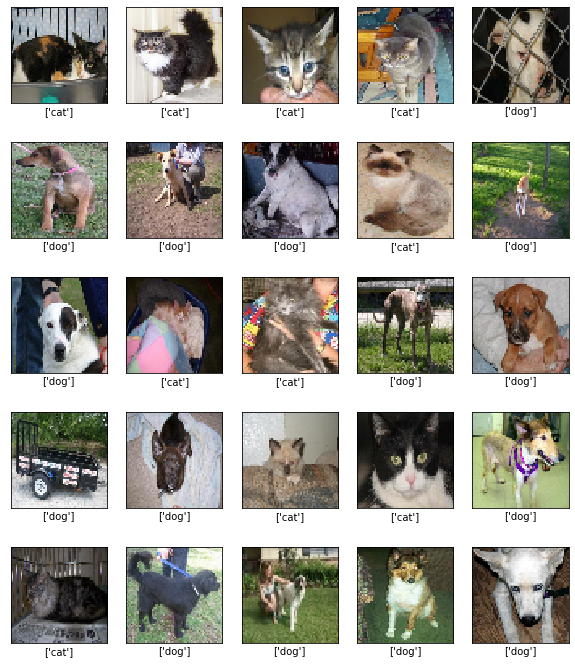
Example Batch

We can iterate once over train_ds_2 to view an example image batch, along with their labels:

image_batch, label_batch = next(iter(train_ds_2))
plt.figure(figsize=(10,12))
for i in range(25):
    plt.subplot(5,5,i+1)
    plt.xticks([])
    plt.yticks([])
    plt.grid(False)
    plt.imshow(image_batch[i], cmap=plt.cm.binary)
    ind = [bool(i) for i in (label_batch[i])]
    plt.xlabel(class_names[ind])
plt.show()

Fitting the Neural Network

We use the keras library, a part of tensorflow, to fit a neural network to classify these images. Most importantly, the Sequential function to build the model and different layer functions to create the neural network layers within the Sequential model build.

from tensorflow.keras.models import Sequential
from tensorflow.keras.layers import Dense, Conv2D, Flatten, Dropout, MaxPooling2D

Below is the code used to specify the model using Sequential.

model = Sequential([
    Conv2D(16, 3, padding='same', activation='relu', 
           input_shape=(image_height, image_width ,3)),
    MaxPooling2D(),
    Dropout(0.2),
    Conv2D(32, 3, padding='same', activation='relu'),
    MaxPooling2D(),
    Conv2D(64, 3, padding='same', activation='relu'),
    MaxPooling2D(),
    Dropout(0.2),
    Flatten(),
    Dense(512, activation='relu'),
    Dense(2)
])

This convolutional neural network contains 8 layers, with a final layer to output a classification. The convolutional layers, given by Conv2D, apply convolutional operations to the image and output a single value based on the operations. The pooling layers, given by MaxPooling2D, extract key features of the image and reduce the dimensionality to reduce computational time. In this case, the max pooling approach extracts the maximum value over subregions of the image. Dropout is another method that helps to reduce overfitting, dropping out a proportion of the dataset, and makes the distribution of weight values in the neural network more regular.

Finally, the Flatten function reformats the data, so that it is vector form and not in a high dimensional format. The Dense layer provides most of the information to the model. These fully connected layers perform the classification on the output to all the other layers. The final Dense(2) will output two nodes, giving probabilities for each one. This will be classifying either a cat or a dog.

This model needs to be compiled. We use the adam optimiser, which is a variation on gradient descent.

model.compile(optimizer='adam',
              loss=tf.keras.losses.BinaryCrossentropy(from_logits=True),
              metrics=['accuracy'])

Now we fit the model.

history = model.fit(
    train_ds_2,
    steps_per_epoch = image_count // batch_size,
    epochs = 10,
    validation_data = val_ds_2,
    validation_steps = image_count_val // batch_size
)

Train for 187 steps, validate for 62 steps
Epoch 1/10
187/187 [==============================] - 22s 119ms/step - loss: 0.6936 - accuracy: 0.5044 - val_loss: 0.6906 - val_accuracy: 0.5514
Epoch 2/10
187/187 [==============================] - 22s 119ms/step - loss: 0.6578 - accuracy: 0.5639 - val_loss: 0.6227 - val_accuracy: 0.6127
Epoch 3/10
187/187 [==============================] - 21s 112ms/step - loss: 0.6024 - accuracy: 0.6527 - val_loss: 0.6277 - val_accuracy: 0.6235
Epoch 4/10
187/187 [==============================] - 21s 113ms/step - loss: 0.5647 - accuracy: 0.6868 - val_loss: 0.5571 - val_accuracy: 0.6920
Epoch 5/10
187/187 [==============================] - 21s 114ms/step - loss: 0.5284 - accuracy: 0.7214 - val_loss: 0.5474 - val_accuracy: 0.7054
Epoch 6/10
187/187 [==============================] - 22s 116ms/step - loss: 0.4949 - accuracy: 0.7411 - val_loss: 0.5419 - val_accuracy: 0.7114
Epoch 7/10
187/187 [==============================] - 21s 114ms/step - loss: 0.4685 - accuracy: 0.7585 - val_loss: 0.5114 - val_accuracy: 0.7384
Epoch 8/10
187/187 [==============================] - 21s 114ms/step - loss: 0.4392 - accuracy: 0.7807 - val_loss: 0.4992 - val_accuracy: 0.7523
Epoch 9/10
187/187 [==============================] - 22s 117ms/step - loss: 0.4091 - accuracy: 0.7996 - val_loss: 0.5721 - val_accuracy: 0.7256
Epoch 10/10
187/187 [==============================] - 21s 113ms/step - loss: 0.3819 - accuracy: 0.8182 - val_loss: 0.4976 - val_accuracy: 0.7573

Evaluating the Model

Now that the model is fit, how do we know that it’s doing a good job? Firstly, by the final lines in the model fitting, we can see that the prediction accuracy ended at around 0.82, so 82% of training set predictions were correct, and around 75% of validation set predicctions were.

We can also plot the loss on the training set and the validation set below. We want this to decrease in both cases, as a smaller loss means a better fit. We also want the predictiona accuracy to increase, so that predictions are more correct. If the validation set loss has also decreased to a low value, and the accuracy has increased, then the model has avoided overfitting.

acc  = history.history['accuracy']
loss = history.history['loss']
val_loss = history.history['val_loss']
val_acc  = history.history['val_accuracy']

epochs_range = range(10)

plt.figure(figsize=(10, 4))
plt.subplot(1, 2, 1)
plt.plot(epochs_range, acc, label='Training Accuracy')
plt.plot(epochs_range, val_acc, label='Validation Accuracy')
plt.legend(loc='lower right')
plt.title('Training and Validation Accuracy')

plt.subplot(1, 2, 2)
plt.plot(epochs_range, loss, label='Training Loss')
plt.plot(epochs_range, val_loss, label='Validation Loss')
plt.legend(loc='upper right')
plt.title('Training and Validation Loss')
plt.show()

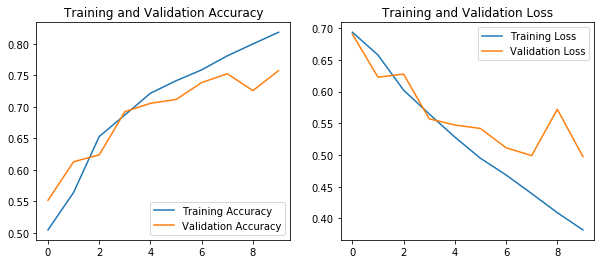
These plots show that the loss steadily decreases, and the accuracy increases in both cases. Now we can evaluate some predictions on the test set. The test set do not have specific class labels, and we are treating these as unknown.

Test Set Predictions

To further test the performance of the model, and inspect it ourselves, we can see how well the model predicts on a test set (which the model has never seen). This is a separate dataset to the validation set which was part of the model fitting process.

Firstly, we load the image using the PIL.Image module, and load the images into a list.

import numpy as np
import PIL.Image as Image
import glob


pred_list = []
for filename in glob.glob('/home/fs19144/Documents/SC2/Section10/data/test/*.jpg'): 
    x = Image.open(filename).resize((image_height, image_width))
    pred_list.append(x)

Next, we loop over the 20 elements in this small test set to inspect the model predictions. Each image is loaded as a numpy array, which automatically converts it into pixel format. These pixel values need to be divided by 255, to get RGB values in $[0,1]$. We obtain model predictions using the simple predict function as part of the model object. These predictions come in terms of fitted values (not strictly probabilities). The predicted classes are then given by taking the largest fitted values output by the model. We can plot the images and their predictions below.

pred_class = np.empty([len(pred_list)], dtype="S3")

plt.figure(figsize=(10,12))
for i in np.arange(len(pred_list)):
    x = np.array(pred_list[i])/255.0
    pred = model.predict(x[np.newaxis, ...])     
    pred_class[i] = class_names[np.argmax(pred[0])]
    
    # Plot
    plt.subplot(4,5,i+1)
    plt.xticks([])
    plt.yticks([])
    plt.grid(False)
    plt.imshow(x)
    plt.xlabel(pred_class[i])

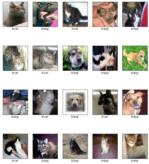
There are some funny looking dogs in this sample, and some funny looking cats. Clearly we can see that oftentimes the model calls a cat a dog, and a dog a cat (I imagine the dogs are more offended by that), but for the most part the predictions look accurate.

There is a lot more that can go into improving this model, such as

• Pre-processing the image data
• Increasing the dataset size
• Increasing the image resolution
• Adding more layers to the neural network
• Adding ‘null’ images, that show neither a cat nor dog, so that the model does not always predict a cat or dog, it can be neither