Numerical Integration

Quadrature

One of the most basic methods to approximate an integral involves collecting a series of shapes or ‘bins’ underneath the a curve, of which the area is known for each bin, and approximating the integral as the sum of the area of these shapes. To do this, we need to estimate the curve for which we are integrating, so we can get points at which to estimate these bins. This can be estimated with polynomial methods. The Weierstrass Approximation Theorem states that there exists a polynomial which can be used to approximate a given continuous function, within a tolerance. More formally, for \(f \in C^0([a,b])\), there exists a sequence of polynomials \(p_n\) that converges uniformly to \(f\) on the interval \([a,b]\), i.e.

\[ ||f-p_n||_{\infty} = \max_{x \in [a,b]} |f(x)-p_n(x)| \to 0. \]

There are many ways to approximate this polynomial, and the obvious way of doing this is by uniformly sampling across the curve, and estimating the polynomial based on these points, but we will show that this is not accurate in most cases. For example, the function \[ f(x) = \frac{1}{50+25\sin{[(5x)^3]}}, \qquad x \in [-1,1] \] has a very complex integral to solve analytically. Wolfram Alpha gives this solution as \[ \int f(x) dx = -\frac{2}{375}i \sum_{\omega:\: \omega^6 - 3\omega^4- 16i\omega^3 + 3\omega^2 - 1=0}\frac{2\omega \tan^{-1}\left( \frac{\sin 5x}{\cos 5x - \omega}\right) - i \omega \log(-2\omega \cos 5x + \omega^2 + 1)}{\omega^4 - 2\omega^2- 8 i \omega +1} , \] which would be an extreme effort to solve without a computer. With quadrature methods, the integral in this one-dimensional case can be approximated with small error due to the Weierstrass Approximation theorem.

We first start by approximating the polynomial \(p_n\) with a basic method of uniformly sampling across the range of \(x\). We can use Lagrange polynomials to approximate the polynomial across these uniform points. A Lagrange polynomial takes the form \[ p_{k-1}(x) := \sum^k_{i=1} \ell_i (x) f_i(x_i), \: \: \: \: \text{ where } \:\:\:\: \ell_i(x) = \prod^k_{j=1, j \neq i} \frac{x-x_j}{x_i-x_j}, \] where \(\ell_i\) are the Lagrange basis polynomials. We start by setting up the function.

x = seq(-1, 1, len=100)
f = function(x) 1/(50+25*sin(5*x)^3)

A Lagrange polynomial function can be set up in R. This function will return an approximating function, of which values of \(x\) can be supplied, just like the original function f is set up.

get_lagrange_polynomial = function(f, x_points){
  function(x){
    basis_polynomials = array(1, c(length(x), length(x_points)))
    for(j in 1:length(x_points)){
      for(m in 1:length(x_points)){
        if(m==j) next
        basis_polynomials[,j] = basis_polynomials[,j] * ((x-x_points[m])/(x_points[j]-x_points[m]))
      }
    }
    p = 0
    for(i in 1:length(x_points)){
      p = p + basis_polynomials[,i]*f(x_points[i])
    }
    return(p)
  }
}

x_points = seq(range(x)[1], range(x)[2], length=30)
lagrange_polynomial = get_lagrange_polynomial(f, x_points)
plot(x, f(x), type="l")
points(x_points, f(x_points), col="red", pch=20)
lines(x, lagrange_polynomial(x), col="red")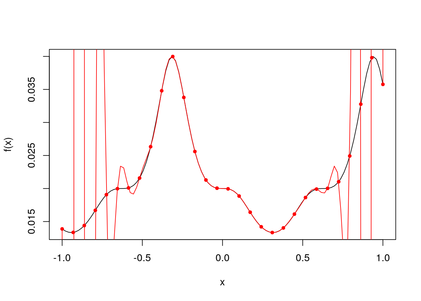

We can see that the Lagrange polynomial approximation approximates the function reasonably well in the middle areas, but the approximation is completely off at the ends. This large deviation is known as Runge’s phenomenon, and this occurs when using polynomial interpolation and equally spaced interpolation points. This can be fixed by using Chebyshev points, which take the form \[ \cos \left(\frac{2i-1}{2k}\pi\right), \] for \(i=1,\dots,k\). This can be simply implented in R.

chebyshev_points = function(k) cos(((2*seq(1,k,by=1)-1)*pi)/(2*k))
c_points = sort(chebyshev_points(30))
lagrange_polynomial = get_lagrange_polynomial(f, c_points)
plot(x, f(x), type="l")
points(c_points, f(c_points), col="red", pch=20)
lines(x, lagrange_polynomial(x), col="red")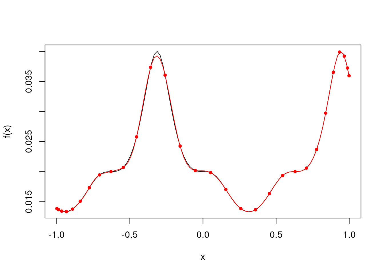

The function is approximated a lot better without any significant deviations from the function. Now that we have a more accurate approximation, we can estimate the area underneath the curve by using a ‘histogram’ approximation to the area. A basic method will simply sum over all small areas of the function evaluation at each point, and the distance between midpoints, i.e. \[ \sum^k_{i=1}w_k f(x_k), \] where \(x_k\) is the \(k\)-th point (calculated with Chebyshev or uniform approximations), and \(w_k\) is the distance between the midpoints above and below point \(x_k\).

hist_approximation = function(f_points, x_points, xrange=c(-1,1)){
  midpoints = (x_points[2:(length(x_points))]+x_points[1:(length(x_points)-1)])/2
  midpoints = c(xrange[1] ,midpoints, xrange[2])
  diffs = diff(midpoints)
  
  sum(diffs*f_points)
}
x_points = seq(range(x)[1], range(x)[2], length=30)
lagrange_polynomial = get_lagrange_polynomial(f, x_points)
hist_approximation(lagrange_polynomial(x_points), x_points)

## [1] 0.04426415

Which we can compare to the analytical solution to the integral. \[ \int^{1}_{-1} \frac{1}{50+25\sin{x}}dx \approx 0.0443078 \] So this isn’t too far off, but can be more approximately calculated with Simpson’s rule, given by \[ \int^b_a f(x) dx \approx \frac{b-a}{6} \left( f(a) + 4f\left(\frac{a+b}{2}\right) + f(b) \right). \] This can be coded into R.

simpsons_approximation = function(f, x_points, xrange=c(-1,1)){
  midpoints = c(xrange[1], x_points, xrange[2])
  diffs = (midpoints[2:(length(midpoints))] - midpoints[1:(length(midpoints)-1)])/6 * (
    f(midpoints[1:(length(midpoints)-1)]) + 4*f((midpoints[2:(length(midpoints))] +
    midpoints[1:(length(midpoints)-1)])/2) + f(midpoints[2:(length(midpoints))])
  )
  
  sum(diffs)
}

c_points = sort(chebyshev_points(30))
simpsons_approximation(get_lagrange_polynomial(f, c_points), c_points)

## [1] 0.044304

This is a closer estimate to the true value. Increasing the number of points increases the accuracy of the integral approximation.

n=1000
ints = rep(NA, (n-10))
for(b in 10:n) {
  c_points = sort(chebyshev_points(b))
  ints[b-10] = simpsons_approximation(f(c_points), c_points)
}
plot(11:n, ints, xlab="No. of Points", log="x", type="l", ylab="Approximated Area")
abline(h=0.0443078, col="red")
legend("topright", col="red", legend="True Integral", lwd=2, lty=1)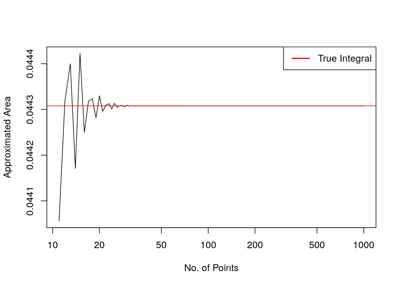

This plot shows that at around 35 points, the accuracy of the integral doesn’t increase significantly.