Introduction

Rcpp sugar and Armadillo are libraries included in Rcpp that allow different processes:

• Sugar provides an array of basic functions in Rcpp that are similar to inbuilt base R functions. These include functions such as cbind, sum, sin, sample and many more. These are essential for writing simple code in Rcpp.
• Armadillo is a package used for linear algebra operations in Rcpp. It allows specification of matrices, 3D matrices, vectors and others.

This portfolio will explain the use of key functions and features of Armadillo and sugar by implementing local polynomial regression on a data set on solar electricity production in Sydney. We can load this data into the R environment first.

load("solarAU.RData")

head(solarAU)

##       prod          toy tod   logprod
## 8832 0.019 0.000000e+00   0 -3.540459
## 8833 0.032 5.708088e-05   1 -3.170086
## 8834 0.020 1.141618e-04   2 -3.506558
## 8835 0.038 1.712427e-04   3 -3.036554
## 8836 0.036 2.283235e-04   4 -3.079114
## 8837 0.012 2.854044e-04   5 -3.816713

The column prod is a production measure, and logprod is the log of the production measure, which will be the response variable. The covariates are toy - the time of year, within 0 and 1 as a percentage, and tod - the time of day, from 0 to 47, measured in half an hour intervals. A simple polynomial regression model is of the form \[ \mathbb{E}(y|\boldsymbol{x}) = \beta_0 + \beta_1\text{tod} + \beta_2\text{tod}^2 + \beta_3\text{toy} + \beta_4 \text{toy}^2 = \tilde{\boldsymbol{x}}\boldsymbol{\beta}. \]

Fitting a linear regression model

We can use Armadillo to fit a linear regression model, and to solve the least squares optimisation problem \[ \hat{\boldsymbol{\beta}} := \operatorname{argmin}_{\boldsymbol{\beta}}\|{\boldsymbol{y}-\boldsymbol{X}\boldsymbol{\beta}\|}^2, \] which has solution \[ \boldsymbol{\hat{\beta}} = (\boldsymbol{X}^T\boldsymbol{X})^{-1}\boldsymbol{X}^T\boldsymbol{y}. \] This can be implemented in C using QR decomposition of \(\boldsymbol{X}\).

library(Rcpp)
sourceCpp(code='
// [[Rcpp::depends(RcppArmadillo)]]
#include <RcppArmadillo.h>
#include <Rcpp.h>
using namespace Rcpp;

// [[Rcpp::export(name="lm_cpp")]]
arma::vec lm_cpp_I(arma::vec& y, arma::mat& X)
{
  arma::mat Q, R;
  arma::qr_econ(Q, R, X);
  arma::vec beta = solve(R, (trans(Q) * y));
  return beta;
}')
ls = function(formula, data){
  y = data[,all.vars(formula)[1]]
  x = model.matrix(formula, data)
  lm_cpp(y, x)
}

Note that the sourceCpp function has a differing argument code, where instead of reading code from a file in the directory, the code is supplied directly here. Running sourceCpp adds the lm_cpp function to the environment. An R function is set up which takes the inputs formula and data and runs the Rcpp function with the given inputs. This makes it comparable to lm. Firstly though, we can see that both functions output the same parameter estimates.

ls(logprod ~ tod + I(tod^2) + toy + I(toy^2), data = solarAU)

##             [,1]
## [1,] -6.26275685
## [2,]  0.86440391
## [3,] -0.01757599
## [4,] -5.91806924
## [5,]  6.14298863

lm(logprod ~ tod + I(tod^2) + toy + I(toy^2), data = solarAU)$coef

## (Intercept)         tod    I(tod^2)         toy    I(toy^2) 
## -6.26275685  0.86440391 -0.01757599 -5.91806924  6.14298863

But which is faster?

microbenchmark(
  R_lm = lm(logprod ~ tod + I(tod^2) + toy + I(toy^2), data = solarAU),
  C_lm = ls(logprod ~ tod + I(tod^2) + toy + I(toy^2), data = solarAU),
  times = 500
)

## Unit: milliseconds
##  expr      min       lq     mean   median       uq      max neval
##  R_lm 3.531021 4.047208 5.079068 4.205777 5.222140 57.54048   500
##  C_lm 2.522135 2.927327 3.615145 3.026044 3.654492 37.26725   500

So the C code is approximately twice as fast with this method, and would be even faster without the R wrapper function. However, the R function lm performs a number of checks and computes a number of statistics that the C++ code does not, which explains part of the performance gap.

For a more fair comparison, we can set up the model matrices in advance, and perform the same operations in R and in RCpp.

R_ls_solve = function(y,X){
  QR = qr(X)
  beta = solve(qr.R(QR), (t(qr.Q(QR)) %*% y))
  return(beta)
}
y = solarAU$logprod
X = with(solarAU, cbind(1, tod, tod^2, toy, toy^2))
microbenchmark(R_solve = R_ls_solve(y,X),
               C_solve = lm_cpp(y, X), 
               times = 500)

## Unit: microseconds
##     expr      min        lq      mean   median        uq       max neval
##  R_solve 1910.686 2189.3570 5022.8070 2464.270 3779.8105 79083.490   500
##  C_solve  449.401  518.7625  690.3906  584.342  687.4495  8261.433   500

So this has come with an approximate speed up of ten times, exemplifying how much more computationally efficient code written in C++ is over R. However, there is a (non-computational) problem with the model. A plot of the residuals from the linear model shows this.

beta = ls(logprod ~ tod + I(tod^2) + toy + I(toy^2), data = solarAU)
res = y - X %*% beta
predplot = ggplot(solarAU, mapping = aes(x=toy, y=tod, z= X%*%beta)) +
  stat_summary_hex() +  xlab("Time of Year") + ylab("Time of Day") +
  theme(legend.title = element_blank())
resplot = ggplot(solarAU, mapping=aes(x=toy, y = tod, z = res)) +
  stat_summary_hex() +  xlab("Time of Year") + ylab("Time of Day") +
  theme(legend.title = element_blank())
grid.arrange(predplot, resplot, ncol=2)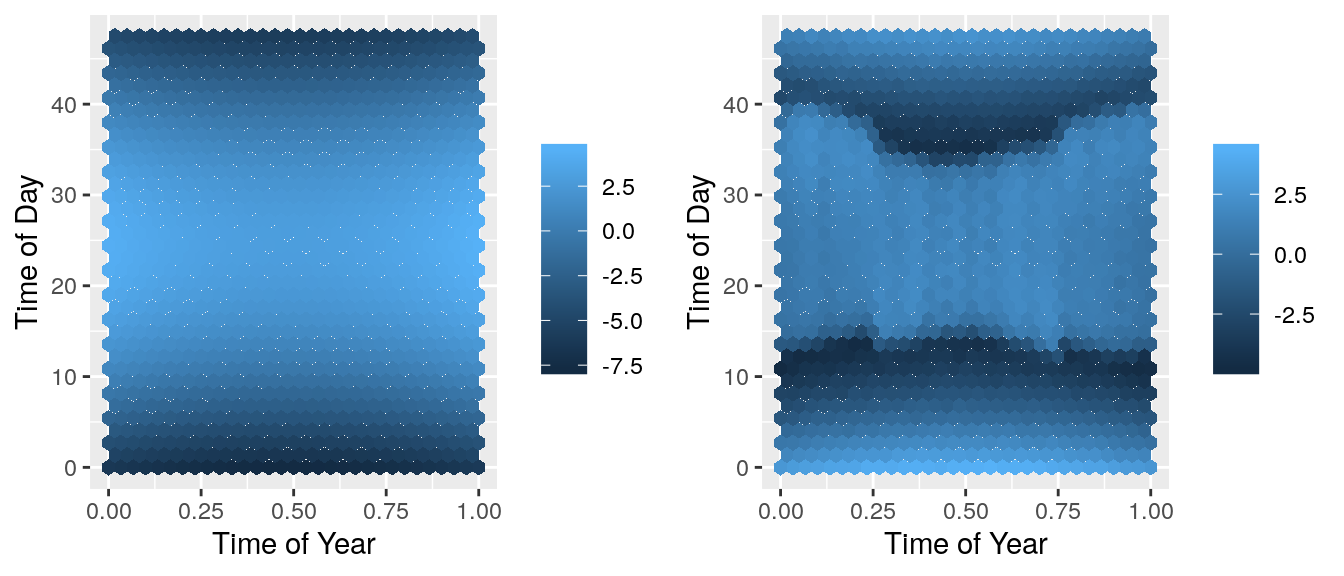

There is a pattern in the residuals! This means that there is a feature not included in the model that can explain some of the noise. We need to extend this model to account for this.

Local Regression

We can improve the model fit by adopting a local regression approach, that is, making the parameter estimates depend on the covariates \(\boldsymbol{x}\), i.e. \(\hat{\boldsymbol{\beta}} = \hat{\boldsymbol{\beta}}(\boldsymbol{x})\). This is achieved by minimising \(\hat{\boldsymbol{\beta}}(\boldsymbol{x}_0)\) for a fixed \(\boldsymbol{x}_0\): \[ \hat{\boldsymbol{\beta}}(\boldsymbol{x}_0) = \operatorname{argmin}_{\boldsymbol{\beta}} \sum^n_{i=1}\kappa_{\boldsymbol{H}}(\boldsymbol{x}_0 - \boldsymbol{x}_i)(y_i-\tilde{\boldsymbol{x}}_i^T\boldsymbol{\beta})^2, \] for a density kernel \(\kappa_{\boldsymbol{H}}\) with positive definite bandwidth matrix \(\boldsymbol{H}\). Fitting this model involves re-fitting the linear model once for each row in the data set, which for large data sets is not viable, but shows the need of computationally efficient code in C++. Now we can write the local regression function in RCpp.

vec local_lm_I(vec& y, rowvec x0, rowvec X0, mat& x, mat& X, mat& H)
{
  mat Hstar = chol(H, "lower"); 
  vec w = dmvnInt(x, x0, Hstar);
  vec beta = lm_cpp_I(y % sqrt(w), X.each_col() % sqrt(w));
  return X0 * beta;
}

// [[Rcpp::export(name="local_lm_fit")]]
vec local_lm_fit_I(vec& y, mat x0, mat X0, mat& x, mat& X, mat& H)
{
  int n0 = x0.n_rows;
  vec out(n0);
  for(int ii=0; ii < n0; ii++)
  {
    rowvec x00 = x0.row(ii);
    rowvec X00 = X0.row(ii);
    out(ii) = as_scalar(local_lm_I(y, x00, X00, x, X, H));
    if(ii % 50 == 0) {R_CheckUserInterrupt();}
  }
  return out;
}

These two functions, as well as lm_cpp from earlier all combine to implement local regression. local_lm_fit_I loops over all rows in x0 and X0 and fits linear regression for a constant \(\boldsymbol{x}_0\), using weights from a Gaussian kernel, imeplemented by a multivariate normal density (given by dmvnInt, defined separately). local_lm_I simply calculates the weights and pre-multiplies them by \(\boldsymbol{y}\) and \(\boldsymbol{X}\) to go into the fitting function. We can source these functions and run these for a subsetted data set.

sourceCpp('lm_cpp.cpp')
nsub = 2000

sub = sample(1:nrow(solarAU), nsub)
y = solarAU$logprod
x = as.matrix(solarAU[c("tod", "toy")])
X = model.matrix(~tod+toy+I(tod^2)+I(toy^2),data=solarAU)
x0 = x[sub, ]
X0 = X[sub, ]
H = diag(c(1,0.01))

cpp_pred_local = local_lm_fit(y, x0, X0, x, X, H)

Of which we can plot, for both the predictions and the residuals.

predPlot = ggplot(mapping=aes(x=x0[,2], y = x0[,1], z = cpp_pred_local)) + stat_summary_hex() +
  xlab("Time of Year") + ylab("Time of Day") + theme(legend.title = element_blank())
resPlot = ggplot(mapping=aes(x=x0[,2], y = x0[,1], z = y[sub] - cpp_pred_local)) + stat_summary_hex() +
  xlab("Time of Year") + ylab("Time of Day") + theme(legend.title = element_blank())
grid.arrange(predPlot, resPlot, ncol=2)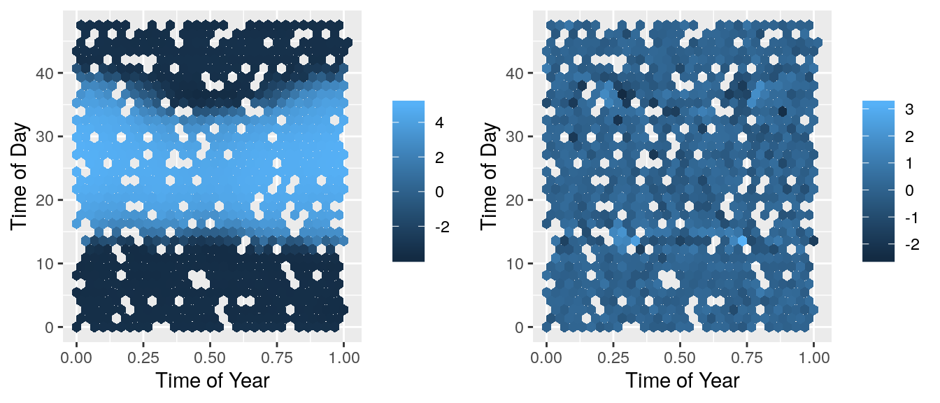

These look a lot better! There isn’t a systematic pattern in these residuals which show that the model isn’t missing anything important. Now we can check this C++ code against the basic R code.

library(mvtnorm)
lmLocal <- function(y, x0, X0, x, X, H){
  w <- dmvnorm(x, x0, H)
  fit <- lm(y ~ -1 + X, weights = w)
  return( t(X0) %*% coef(fit) )
}
R_pred_local <- sapply(1:nsub, function(ii){
  lmLocal(y = y, x0 = x0[ii, ], X0 = X0[ii, ], x = x, X = X, H = diag(c(1, 0.1)^2))
})

all.equal(R_pred_local, as.vector(cpp_pred_local))

## [1] TRUE

Since all these predictions are equal in R and Rcpp, how does the speed difference compare? This function takes a long time to run, so we will only time each of them once.

system.time(sapply(1:nsub, function(ii){
  lmLocal(y = y, x0 = x0[ii, ], X0 = X0[ii, ], x = x, X = X, H = diag(c(1, 0.1)^2))
}))

##    user  system elapsed 
##  23.527   0.076  23.606

system.time(
  local_lm_fit(y, x0, X0, x, X, H)
)

##    user  system elapsed 
## 872.113   0.309 145.901

So the Rcpp code has come with an approximate ten times speed up again. However, this model could still be improved. We have chosen the bandwidth matrix \(\boldsymbol{H}\) arbitrarily, but this could be improved with cross-validation. Whilst this is not shown here, a similar approach to that given in section 2 could be implemented.