Introduction to Python for Statistics
Introduction
Python is a powerful programming language that is very popular for data analysis as well as many other applications in the real world. This portfolio will go over some intermediary processes in Python 3.7.3, before implementing basic statistical models; including linear models, regression and classification.
Python Overview
Functions and Modules
Similar to R, functions can be defined and called in the same script. The function definition syntax is as follows
def function_name(input1, input2):
    variable = function_operation
    second_variable = second_function_operation
    return output
There’s a couple things to note here. Firstly, indentation is essential to defining the function. Unlike R or MATLAB, there is nothing to write that marks the beginning or end of the function as this is all handled by where the indentation begins and ends. Secondly, the function name comes after the def, instead of the other way around (as in R). Finally, the colon (:) is necessary, as it is in loops and if statements.
Functions can be written in one script, and called in another, and the way this is achieved is through modules. Modules are a collection of code that you can load from another file, similar to how source and library work in R. You load modules with any of these lines:
import module_name
import module_name as short_name
from module_name import function_name
from module_name import *
All these commands load the module (or parts of it), but do it slightly differently. In Python, all modules loaded have to be accessed through their name to use their functions. For example, to use a function from NumPy, you would have to use numpy.function_name. This name can be shortened if you used the second line above to load the module, commonly, NumPy is abbreviated to np so that you would only have to type np.function_name to access it.
You can also load specific functions from a module by using the third and fourth line above, where the asterisk * indicates to load all functions from the module. Note that if the module is loaded this way, you do not need to specify the name of the module preceding the function. It is considered bad practice to load functions this way, as declaring the module name removes the chance of overlapping function names within modules.
Example: Morse Code
As an example of basic operations in Python, consider writing two functions to encode and decode morse code respectively. The encoding function will take a string, or a piece of text, and convert it into morse code. The decoding function does the opposite: converts morse code into plain english text. To write these functions, we first must define a dictionary:
letter_to_morse = {'a':'.-', 'b':'-...', 'c':'-.-.', 'd':'-..', 'e':'.',
        'f':'..-.', 'g':'--.', 'h':'....', 'i':'..', 'j':'.---', 'k':'-.-',
        'l':'.-..', 'm':'--', 'n':'-.', 'o':'---', 'p':'.--.', 'q':'--.-',
        'r':'.-.', 's':'...', 't':'-', 'u':'..-', 'v':'...-', 'w':'.--',
        'x':'-..-', 'y':'-.--', 'z':'--..', '0':'-----', '1':'.----',
        '2':'..---', '3':'...--', '4':'....-','5':'.....', '6':'-....',
        '7':'--...', '8':'---..', '9':'----.', ' ':'/'}
So this dictionary can be accessed by indexing with the letter that we want a translation for. For example
letter_to_morse["6"]
Likewise, we need to define the reverse; a dictionary that takes morse code and outputs an english letter. We can reverse this dictionary with a loop.
morse_to_letter = {}
for letter in letter_to_morse:
    morse = letter_to_morse[letter]
    morse_to_letter[morse] = letter
morse_to_letter[".-"]
Now we can define the two functions encode and decode that use these two dictionaries. For the encoding function:
def encode(x):
    morse = []
    for letter in x:
        letter = letter.lower()
        morse.append(letter_to_morse[letter])

    morse_message = " ".join(morse)
    return morse_message
This function initialises an array morse, and loops over all letters in the input x and appends to the morse array the translation in morse code. After the loop, the morse array is joined together. For the decoding function:
def decode(x):
    english = []
    morse_letters = x.split(" ")
    for letter in morse_letters:
        english.append(morse_to_letter[letter])

    english_message = "".join(english)
    return english_message
This has a similar process as with encode. First the input x is split, and then each split morse symbol is looped over and converted to english using the morse_to_letter dictionary. Before we run these functions, we can save them in a separate file called morse.py and put it in our working directory. Then using another script (which will be called run_morse.py), we can import the morse.py functions as a module.
So we can import morse and run the decode function.
import morse
morse_message = ".... . .-.. .--. / .. -- / - .-. .- .--. .--. . -.. / .. -. / ... --- -- . / -- --- .-. ... . / -.-. --- -.. ."
morse.decode(morse_message)
Likewise, we can encode a secret message using morse.encode:
morse.encode("please dont turn me into morse code")
One thing to note here is that the dictionaries morse_to_letter and letter_to_morse were defined outside of the functions. Since this module was imported, we can actually access this:
morse.letter_to_morse
Although oftentimes we would want variables to remain hidden, this is not possible if we are importing all the contents of a script. Importing Python files as modules is usually done so that functions can be imported across the working directory, as opposed to having one big file that contains all the code.
Classes
Object oriented programming in Python is done through classes, the general form of which is
class class_name:
      def __init__(self):
          self.variable_I_want_to_define = variable
          self.another_variable_I_want_to_define = variable_2
      def some_class_function(self, x):
          something_I_can_do_with_my_variables = x
          return some_output
      def some_other_function(self):
          self.an_internal_variable = 3
          return another_output
The functions can be run as a member of the class, and the __init__(self) section of the class is a function that is run when the class is initialised. Any variables that are within the __init__ section of the class become defined, sometimes depending on the inputs to the __init__ function. These could be variables such as initial conditions, or initial estimates. We could add more inputs to the __init__ function after self, if needed.
The other functions can be called, and these could change some of the internal self. variables, e.g. updating the initial conditions, running a certain loop or adding additional variables.
Example: Morse Code Again
We can update the morse code example to write a class called morse_code_translator that has an encode and decode function as part of the class. This is written as
class morse_code_translator:
      def __init__(self):
          self.letter_to_morse = {'a':'.-', 'b':'-...', 'c':'-.-.', 'd':'-..',
            'e':'.', 'f':'..-.',  'g':'--.', 'h':'....', 'i':'..', 'j':'.---',
            'k':'-.-', 'l':'.-..', 'm':'--', 'n':'-.', 'o':'---', 'p':'.--.',
            'q':'--.-', 'r':'.-.', 's':'...', 't':'-', 'u':'..-', 'v':'...-',
            'w':'.--', 'x':'-..-', 'y':'-.--', 'z':'--..', '0':'-----',
            '1':'.----', '2':'..---', '3':'...--', '4':'....-', '5':'.....',
            '6':'-....', '7':'--...', '8':'---..', '9':'----.', ' ':'/'}
          self.morse_to_letter = {}
          for letter in self.letter_to_morse:
              morse = self.letter_to_morse[letter]
              self.morse_to_letter[morse] = letter
          self.english_message_history = []
          self.morse_message_history = []
      def encode(self, x):
          morse = []
          for letter in x:
              letter = letter.lower()
              morse.append(self.letter_to_morse[letter])
          morse_message = " ".join(morse)
          self.english_message_history.append(x)
          self.morse_message_history.append(morse_message)
          return morse_message
      def decode(self, x):
          english = []
          morse_letters = x.split(" ")
          for letter in morse_letters:
              english.append(self.morse_to_letter[letter])
          english_message = "".join(english)
          self.english_message_history.append(english_message)
          self.morse_message_history.append(x)
          return english_message
So this has simply moved the decode and encode functions over inside a class. The dictionaries are now written as self.letter_to_morse and self.morse_to_letter, with the self. prefix. Other than that, I have also added two more variables: english_message_history and morse_message_history, to exemplify how variables can be updated by calling the functions. Every time encode or decode is run, these arrays keep track of all messages that have passed through either function. We can test to see if this works, by importing this class from morse_class.py.
from morse_class import morse_code_translator
translator = morse_code_translator()
translator.encode("please not again")
translator.decode(".--. .-.. . .- ... . / -.. --- -. - / - ..- .-. -. / -- . / .. -. - --- / . -. --. .-.. .. ... ....")
So this has worked as expected, and the translator object now can both decode and encode morse code messages. Now that these two messages have passed through the class, we can see if the history has worked.
translator.english_message_history
translator.morse_message_history
So the internal self variables have been updated with the two messages that were passed through the class.
Statistical Models
Python has a lot of support for fitting statistical models and machine learning, this is mostly as part of the sklearn package. Other modules must also be imported that provide different funtionality. Statistical models are handled by sklearn, dataframes are handled by pandas and numpy, randomness is handled by numpy and random, and plots are handled by matplotlib.
import sklearn as sk
import sklearn.linear_model as lm
import pandas as pd
import numpy as np
import random
import matplotlib.pyplot as plt
Linear Regression
A basic linear regression model in python is handled as part of the sklearn.linear_model module. The use of a linear model in Python can be explained through an example. Some simulated data can be set up as follows
$$
\boldsymbol{x} \sim \text{Unif}(0,1), \qquad y \sim N(\boldsymbol{\mu}, .5), \qquad \boldsymbol{\mu} = \beta_0 + \beta_1 \boldsymbol{x},
$$
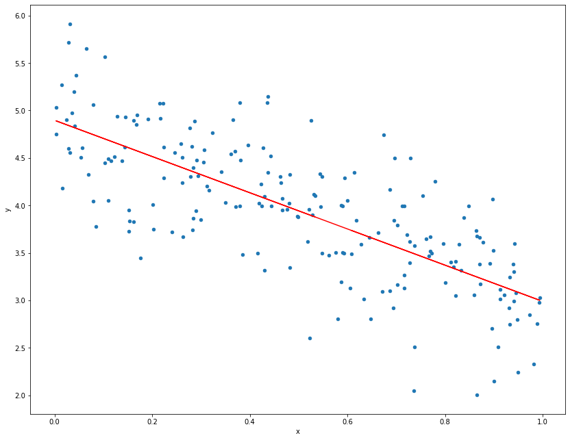
where both $\boldsymbol{x}$ and $\boldsymbol{y}$ are of length $n$. Since this is simulated data, we pre-define $\beta_0 = 5$ and $\beta_1 = -2$ as the intercept and the gradient. We can use numpy to sample this data, and the linear_model module in sklearn to fit a linear model to it.
n = 200
beta0 = 5
beta1 = -2
x = np.random.uniform(0, 1, n)
mu = beta0 + beta1*x
y = np.random.normal(mu, .5, n)
This data can be converted into a dataframe with the DataFrame function in pandas.
data = pd.DataFrame({"x":x, "y":y})
To set up the linear model, a model object must be set up in advance, and then the fitting routine can be called to it. This can be done in one line by nesting operations.
model = lm.LinearRegression(fit_intercept=True).fit(data[["x"]], data["y"])
Here, the model has been fit by first creating a linear model object with lm.LinearRegression (and specifying that we do want an intercept). Secondly, the .fit() function has been called on that object to obtain parameter estimates $\beta_0$ and $\beta_1$ by passing the covariates x and response variable y to it. Now we can see whether these estimates bare resemblance to the true parameter values used to simulate the data.
print("Intercept:", model.intercept_, ",", "Gradient:", model.coef_)
Intercept: 4.89676478340633 , Gradient: [-1.90845212]
This is reasonably close to the true values. Note that here there is only one covariate vector, but this method is applicable to multiple covariates which would give multiple estimates of the gradient for each covariate. Now we can plot the data and the fit, a pandas data frame has an inbuilt method used for plotting the data, which produces a scatter plot from matplotlib.
data.plot.scatter("x", "y", figsize=(14, 11));
plt.plot(x, model.predict(data[["x"]]), 'r');
Multiple Linear Regression
In the previous section, we fit a linear model with a single covariate vector. This is good for exemplary purposes as a two dimensional linear model is easy to visualise. Often in data analysis we can have multiple explanatory variables $\boldsymbol{x}_1, \dots, \boldsymbol{x}_p$ that give information about the respone variable $\boldsymbol{y}$.
For an example of multiple linear regression, we will be using the Boston house prices dataset, which is part of the freely provided datasets from sklearn. This dataset describes the median value of owner-occupied homes (per $1000), as well as 13 predictors that could provide information about the house value. We load this dataset and convert it to a pandas data frame.
from sklearn.datasets import load_boston
data = load_boston()
boston = pd.DataFrame(data.data, columns = data.feature_names)
boston["MEDV"] = data.target
boston.head()
| CRIM | ZN | INDUS | CHAS | NOX | RM | AGE | DIS | RAD | TAX | PTRATIO | B | LSTAT | MEDV | |
|---|---|---|---|---|---|---|---|---|---|---|---|---|---|---|
| 0 | 0.00632 | 18.0 | 2.31 | 0.0 | 0.538 | 6.575 | 65.2 | 4.0900 | 1.0 | 296.0 | 15.3 | 396.90 | 4.98 | 24.0 |
| 1 | 0.02731 | 0.0 | 7.07 | 0.0 | 0.469 | 6.421 | 78.9 | 4.9671 | 2.0 | 242.0 | 17.8 | 396.90 | 9.14 | 21.6 |
| 2 | 0.02729 | 0.0 | 7.07 | 0.0 | 0.469 | 7.185 | 61.1 | 4.9671 | 2.0 | 242.0 | 17.8 | 392.83 | 4.03 | 34.7 |
| 3 | 0.03237 | 0.0 | 2.18 | 0.0 | 0.458 | 6.998 | 45.8 | 6.0622 | 3.0 | 222.0 | 18.7 | 394.63 | 2.94 | 33.4 |
| 4 | 0.06905 | 0.0 | 2.18 | 0.0 | 0.458 | 7.147 | 54.2 | 6.0622 | 3.0 | 222.0 | 18.7 | 396.90 | 5.33 | 36.2 |
The variable we are interested in predicting is MEDV, and all other variables will be used to give information to predicting MEDV.
Before fitting any models, we can perform some exploratory data analysis to help the decision as to what predictor variables need to be included in the model fitting. Luckily, there are easy methods available that inspect how strongly correlated variables are with other variables in a pandas data frame. Firstly, we will be using the inbuilt corr function and plotting it as a heatmap. This uses the seaborn module to create a heatmap.
import seaborn
corr = boston.corr()
cmap = seaborn.diverging_palette(-500, -720, as_cmap=True)
plt.figure(figsize=(14, 11))
seaborn.heatmap(corr, cmap=cmap);
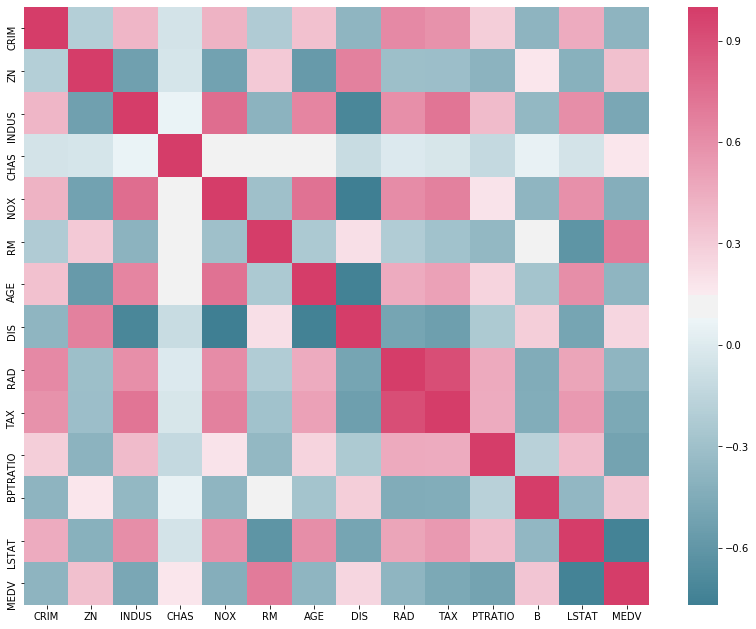
There are two things to infer from this plot: how correlated the predictor variables are from one another, and how correlated the predictor variables are from the response. We are mostly interested in how correlated the predictors are with MEDV, as if they influence the value of MEDV significantly, then they are likely to be important to include in a model. Another plot we can use to explore the data is a multi variable scatter plot. That is, a scatter plot for each pair of variables. pandas has a function for this, as part of the plotting submodule.
from pandas.plotting import scatter_matrix
scatter_matrix(boston, figsize=(16, 16));

There is a lot to process in this plot, but you can restrict your attention to the final column on the right. This column will show scatter plots with all predictor variables and the response MEDV. We are looking for obvious relationships between the two variables. CRIM seems to have an effect at lower values, ZN seems to have a small effect, INDUS has a non-linear relationship,RM has a clear linear relationship, AGE seems to have a significant effect at lower values, B has an effect at larger values and LSTAT seems to have a quadratic relationship. These variables will be important to consider, but that does not mean all others are not. Since some of these predictors are categorical (even binary), it can be hard to infer their relationship with MEDV from a scatter plot.
We can now fit the model using the information above. The predictors we want to include are CRIM, ZN, INDUS, RM, AGE, B and LSTAT. We use the linear model from sklearn again, but first create the new data frame of the reduced dataset. Additionally we can include a quadratic effect for certain predictors by creating a new column in the data frame with the squared values.
boston_x = boston[["CRIM", "ZN", "INDUS", "RM", "AGE", "B", "LSTAT"]]
boston_x.insert(len(boston_x.columns), "LSTAT2", [i**2 for i in boston_x["LSTAT"] ])
boston_x.insert(len(boston_x.columns), "AGE2", [i**2 for i in boston_x["AGE"] ])
boston_x.insert(len(boston_x.columns), "B2", [i**2 for i in boston_x["B"] ])
Now using the linear model with this modified data frame to fit the full model.
mv_model = lm.LinearRegression(fit_intercept=True).fit(boston_x, data.target)
print("Intercept: \n", mv_model.intercept_, "\n")
print("Coefficients:")
print(" \n".join([str(boston_x.columns[i]) + " " + str(mv_model.coef_[i]) for i in np.arange(len(mv_model.coef_))]))
Intercept:
 5.916804277809813

Coefficients:
CRIM -0.11229848683846888
ZN 0.0037476008537828498
INDUS -0.0021805395766587208
RM 4.0621316253156285
AGE 0.07875634757295602
B 0.042639346099976716
LSTAT -2.063750521016358
LSTAT2 0.042240400122337596
AGE2 -0.0002509463690499019
B2 -7.788232883181183e-05
Penalised Regression
The linear_model submodule of sklearn doesn’t just contain the LinearRegression object, it contains many other variations of linear models. Some examples of these are penalised regression models, such as the Lasso model or ridge regression model. You can view the documentation for these online, and they work similarly to LinearRegression. Below I will briefly go through an example of using a Lasso path algorithm on the dataset provided above. Firstly, the model object can be created immediately using the linear_model.lars_path object.
_,_,coefs = lm.lars_path(data.data, data.target)
This is using the full dataset provided in data.data, as the Lasso path plot can be used for feature selection, similar to the scatter matrix approach above.
xx = np.sum(np.abs(coefs.T), axis=1)
xx /= xx[-1]
plt.figure(figsize=(16, 9))
plt.plot(xx, coefs.T)
ymin, ymax = plt.ylim()
plt.vlines(xx, ymin, ymax, linestyle='dashed')
plt.xlabel('|coef| / max|coef|')
plt.ylabel('Coefficients')
plt.title('LASSO Path')
plt.axis('tight')
plt.legend(data.feature_names)
plt.show()
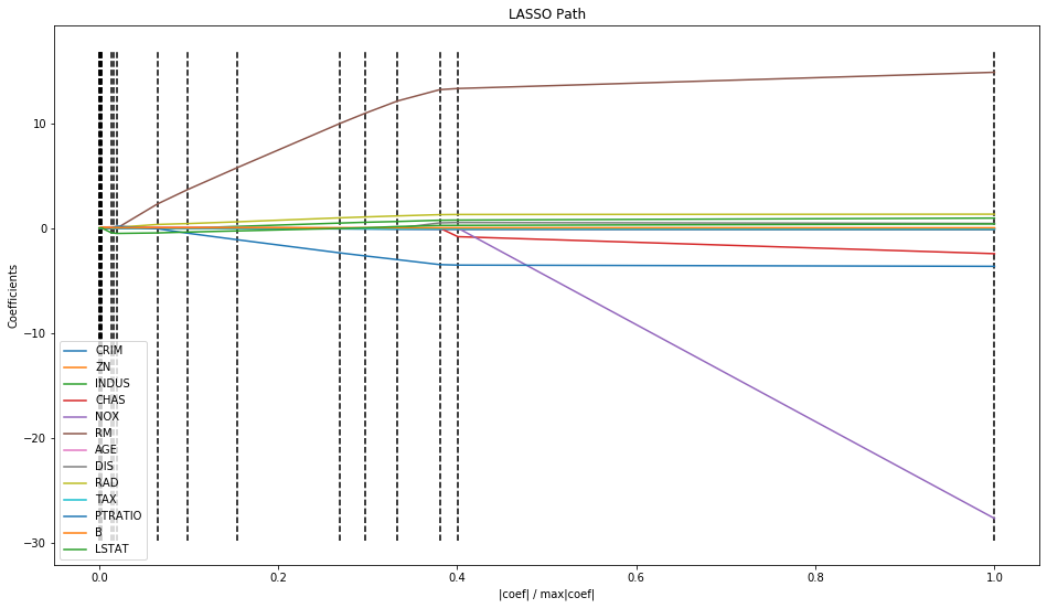
The coefficients for covariates that provide a lot of information to the response variable are likely going to take a very large value of regularisation parameter to shrink them to zero. These are the lines that are more separated in the plot above, i.e. CRIM, RM, NOX, and CHAS. Interestingly, these were not the variables that were selected in the scatter matrix approach earlier in this report, highlighting the variation in parameter selection depending on the method.
Classification
The final statistical model introduced will be one interested in classifying. Classification is interested in prediction of a usually non-numeric class, i.e. assign the output to a pre-defined class based on some inputs. The classification model explained here will be Logistic Regression (ignore the name, it’s not a regression method).
Logistic regression is called so because it uses a logistic function to map fitted values to probabilities. The basic form of a classification model is the same of that of a regression method, except the output from the model corresponds to latent, unobserved fitted values which decide the class of each set of inputs.
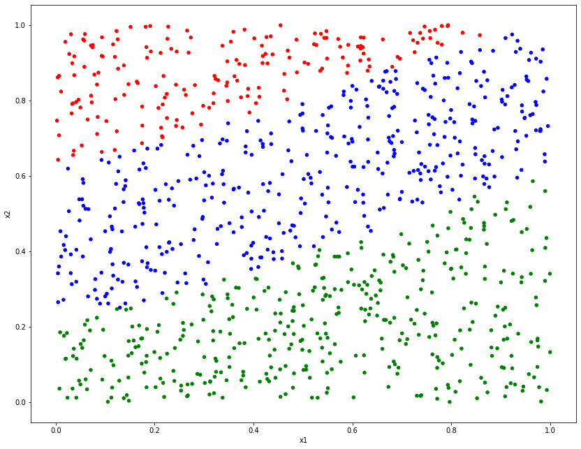
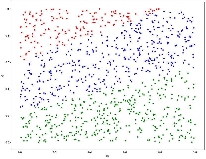
We will start by simulating some data $\boldsymbol{y}$ that need to be classified, which will be generated by a mathematical combination of some inputs $\boldsymbol{x}$. Each element of $\boldsymbol{y}$ will be given one of the class labels $\mathcal{C}_1$, $\mathcal{C}_2$ or $\mathcal{C}_3$. The goal of the statistical model is parameter estimation, similar to the regression methods.
# Simulate x
n = 1000
x1 = np.random.uniform(0, 1, n)
x2 = np.random.uniform(0, 1, n)

# Create parameters and mean
beta0 = 3
beta1 = 1.5
beta2 = -4.8
beta3 = 0.5
mu = beta0 + beta1*x1 + beta2*x2 + beta3*x1**2

# Set class based on value of mean
y = np.repeat("Class 1", n)
y[mu > 0] = "Class 2"
y[mu > 2] = "Class 3"

# Combine into DataFrame
clsf_dat = pd.DataFrame({"y":y,"x1":x1,"x2":x2 })
colors = y
colors[y == "Class 1"] = "red"
colors[y == "Class 2"] = "blue"
colors[y == "Class 3"] = "green"
clsf_dat.plot.scatter("x1", "x2", c=colors, figsize=(14, 11));
Now that the data is set up, we can fit the logistic regression model to it. LogisticRegression is a function as part of the linear_model submodule of sklearn, just as before, so this next step should be familiar to you.
lr_model = lm.LogisticRegression(fit_intercept=True, solver='newton-cg', multi_class = 'auto')
lr_model = lr_model.fit(clsf_dat[["x1", "x2"]], clsf_dat["y"])
print("Intercept: \n", lr_model.intercept_, "\n")
print("Coefficients:")
print(" \n".join([str(clsf_dat.columns[i]) + " " + str(lr_model.coef_[i]) for i in np.arange(len(lr_model.coef_))]))
Intercept:
 [-4.45432353  0.92640783  3.52791569]

Coefficients:
y [-4.06694321  9.66044839]
x1 [0.18794764 0.76440687]
x2 [  3.87899558 -10.42485527]
Note that there are multiple coefficients for each input! This is because even though the data were simulated using one parameter each, the logistic regression model has a different input combination for each class. The first class has both coefficients aliased to the intercept, and anything significantly different (in line with the combination of the remaining parameters) is given a different class.
We can roughly evaluate the model’s performance by inspecting a plot of its predictions.
predictions = lr_model.predict(clsf_dat[["x1", "x2"]])
colors = predictions
colors[predictions == "Class 1"] = "red"
colors[predictions == "Class 2"] = "blue"
colors[predictions == "Class 3"] = "green"
clsf_dat.plot.scatter("x1", "x2", c=colors, figsize=(14, 11));
Here we can see an extremely similar plot to the one above, although it is not quite exactly the same! At the point of overlap between classes, some points are mislabelled as the wrong class, due to uncertainty around the decision boundaries.
More complex models exist for classification and regression, but that’s for another time.