Optimisation

Optimising a complicated function

To demonstrate the different optimisation methods, the speeds and abilities of each, consider optimising the Rastrigin function. This is a non-convex function that takes the form \[ f(\boldsymbol{x}) = An + \sum^n_{i=1} [x_i^2-A\cos(2\pi x_i)], \]

where \(n\) is the length of the vector \(\boldsymbol{x}\). We can plot this function in 3D using the plotly package to inspect it.

f = function(x) A*n + sum(x^2 - A*cos(2*pi*x))
A = 5
n = 2
x1 = seq(-10,10,length=100)
x2 = seq(-10,10,length=100)
xy = expand.grid(x1,x2)
z = apply(xy,1,f)
dim(z) = c(length(x1),length(x2))
z.plot = list(x=x1, y=x2, z=z)
image(z.plot, xlab = "x", ylab = "y", main = "Rastrigin Function")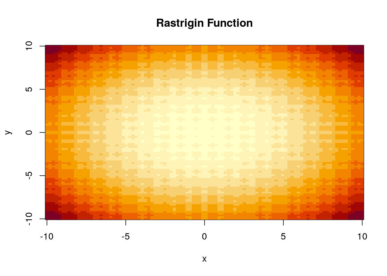

So we are interested in optimising the function f. We can see from inspection of the plot that there is a global minimum at \(\boldsymbol{x} = \boldsymbol{0}\), where \(f(\boldsymbol{0}) = 0\), and likewise:

f(c(0,0))

## [1] 0

So we will be evaluating optimisation methods based on how close they get to this true solution. We continue this portfolio by explaining the different optimisation methods, and evaluating their performance in finding the global minimum of the Rastrigin function.

When \(n=2\), the gradient and hessian for this function can be calculated analytically: \[ \nabla f(\boldsymbol{x}) = \begin{pmatrix} 2 x_1 + 2\pi A \sin(2\pi x_1) \\ 2 x_2 + 2\pi A \sin(2\pi x_2) \end{pmatrix} \] \[ \nabla^2 f(\boldsymbol{x}) = \begin{pmatrix} 2 + 4\pi^2 A \cos (2\pi x_1) & 0 \\ 0 & 2 + 4\pi^2 A \cos (2\pi x_2) \end{pmatrix} \] We can construct these functions in R.

grad_f = function(x) {
  c(2*x[1] + 2*pi*A*sin(2*pi*x[1]),
    2*x[2] + 2*pi*A*sin(2*pi*x[2]) )
}
hess_f = function(x){
  H11 = 2 + 4*pi^2*A*sin(2*pi*x[1])
  H22 = 2 + 4*pi^2*A*sin(2*pi*x[2])
  return(matrix(c(H11,0,0,H22),2,2))
}

These analytical forms of the gradient and hessian can be supplied to various optimisation algorithms to speed up convergence.

Optimisation problems can be one or multi dimensional, where the dimension refers to the size of the parameter vector, in our case \(n\). Generally, one-dimensional problems are easier to solve, as there is only one parameter value to optimise over. In statistics, we are often interested in multi-dimensional optimisation. For example, in maximum likelihood estimation we are trying to find parameter values that maximise a likelihood function, for any number of parameters. For the Rastrigin function in our example, we have taken the dimension \(n=2\).

Gradient Descent Methods

Iterative algorithms take the form \[ \boldsymbol{x}_{k+1} = \boldsymbol{x}_k + t \boldsymbol{d}_k, \: \: \text{ for iterations } k=0,1,\dots, \] \(\boldsymbol{d}_k \in \R^n\) is the descent direction, \(t_k\) is the stepsize. \[ f'(\boldsymbol{x}; \boldsymbol{d})=\nabla f(\boldsymbol{x})^T \boldsymbol{d} < 0. \] So moving \(\boldsymbol{x}\) in the descent direction for timestep \(t\) decreases the function, so we move towards a minimum. The is the negative gradient of \(f\), i.e. \(\boldsymbol{d}_k = -\nabla f(\boldsymbol{x}_k)\), or normalised \(\boldsymbol{d}_k = {-\nabla f(\boldsymbol{x}_k)}/{\norm{\nabla f(\boldsymbol{x})}}\). We can construct a general gradient descent method in R and evaluate performance on optimising the Rastrigin function.

gradient_method = function(f, x, gradient, eps=1e-4, t=0.1, maxiter=1000){
  converged = TRUE
  iterations = 0
  while((!all(abs(gradient(x)) < eps))){
    if(iterations > maxiter){
      cat("Not converged, stopping after", iterations, "iterations \n")
      converged = FALSE
      break
    }
    gradf = gradient(x)
    d = -gradf/abs(gradf)
    x = x - t*gradf
    iterations = iterations + 1
  } 
  if(converged) {cat("Number of iterations:", iterations, "\n")
                 cat("Converged!")}
  return(list(f=f(x),x=x))
}

This code essentially will continue running the while loop until the tolerance condition is satisfied, where the change in \(\boldsymbol{x}\) from one iteration to another is negligible. Now we can see in which cases this will provide a solution to the problem of the Rastrigin function.

gradient_method(f, x = c(1, 1), grad_f)

## Not converged, stopping after 1001 iterations

## $f
## [1] 20.44268
## 
## $x
## [1] -3.085353 -3.085353

gradient_method(f, x = c(.01, .01), grad_f)

## Not converged, stopping after 1001 iterations

## $f
## [1] 17.82949
## 
## $x
## [1] -2.962366 -2.962366

Even when the initial guess of \(x\) was very close to zero, the true solution, this function did not converge. This shows that under a complex and highly varying function such as the Rastrigin function, the gradient method has problems. This can be improved by including a backtracking line search to dynamically change the value of the stepsize \(t\) to \(t_k\) for each iteration \(k\). This method reduces the stepsize \(t\) for each iteration \(k\) via \(t_k = \beta t_k\) for \(\beta \in (0,1)\) while \[ f(\boldsymbol{x}_k) - f(\boldsymbol{x}_k + t_k \boldsymbol{d}_k) < -\alpha\nabla f(\boldsymbol{x}_k)^T \boldsymbol{d}_k. \] and for \(\alpha \in (0,1)\). We can add this to the gradient method function with the line while( (f(x) - f(x + t*d) ) < (-alpha*t * t(gradf)%*%d)) t = beta*t. Meaning we need to specify \(\alpha\) and \(\beta\). After this is added to the function, we have

gradient_method(f, c(0.01,0.01), grad_f, maxiter = 10000)

## Number of iterations: 1255 
## Converged!

## $f
## [1] 5.002503e-09
## 
## $x
## [1] 5.008871e-06 5.008871e-06

Now we finally have convergence! However, this is for when the initial guess was very close to the actual solution, and so in more realistic cases where we don’t know this true solution, this method is likely inefficient and inaccurate. The Newton method is an advanced form of the basic gradient descent method.

Newton Methods

The Newton method seeks to solve the optimisation problem using evaluations of Hessians and a quadratic approximation of a function \(f\) around \(\boldsymbol{x}_k\). This is under the assumption is that the Hessian \(\nabla^2 f(\boldsymbol{x}_k)\) is . The unique minimiser of the quadratic approximation is \[ \boldsymbol{x}_{k+1} = \boldsymbol{x}_k - (\nabla^2 f(\boldsymbol{x}_k))^{-1} \nabla f(\boldsymbol{x}_k), \] which is known as . Here you can consider \((\nabla^2 f(\boldsymbol{x}_k))^{-1} \nabla f(\boldsymbol{x}_k)\) as the descent direction in a scaled gradient method. The nlm function from base R uses the Newton method. It is an expensive algorithm to run, because it involves inverting a matrix, the hessian matrix of \(f\). Newton methods work a lot better if you can supply an algebraic expression for the hessian matrix, so that you do not need to numerically calculate the gradient on each iteration. We can use nlm to test the Newton method on the Rastrigin function.

f_fornlm = function(x){
  out = f(x)
  attr(out, 'gradient') <- grad_f(x)
  attr(out, 'hessian') <-  hess_f(x)
  return(out)
}
nlm(f, c(-4, 4), check.analyticals = TRUE)

## $minimum
## [1] 3.406342e-11
## 
## $estimate
## [1] -4.135221e-07 -4.131223e-07
## 
## $gradient
## [1] 1.724132e-05 1.732303e-05
## 
## $code
## [1] 2
## 
## $iterations
## [1] 3

So this converged to the true solution in a surprisingly small number of iterations. The likely reason for this is due to Newton’s method using a quadratic approximation, and the Rastrigin function taking a quadratic form.

BFGS

In complex cases, the hessian cannot be supplied analytically. Even if it can be supplied analytically, in high dimensions the hessian is a very large matrix, which makes it computationally expensive to invert for each iteration. The BFGS method approximates the hessian matrix, increasing computability and efficiency. The BFGS method is the most common quasi-Newton method, and it is one of the methods that can be suppled to the optim function. It approximates the hessian matrix with \(B_k\), and for iterations \(k=0,1,\dots\), it has the following basic algorithm:

Initialise \(B_0 = I\) and initial guess \(x_0\).

1. Obtain a direction \(\boldsymbol{d}_k\) through the solution of \(B_k \boldsymbol{d}_k = - \nabla f(\boldsymbol{x}_k)\)
2. Obtain a stepsize \(t_k\) by line search \(t_k = \text{argmin} f(\boldsymbol{x}_k + t\boldsymbol{d}_k)\)
3. Set \(s_k = t_k \boldsymbol{d}_k\)
4. Update \(\boldsymbol{x}_{k+1} = \boldsymbol{x}_k + \boldsymbol{s}_k\)
5. Set \(\boldsymbol{y}_k = \nabla f(\boldsymbol{x}_{k+1}) - \nabla f(\boldsymbol{x}_k)\)
6. Update the hessian approximation \(B_{k+1} = B_k + \frac{\boldsymbol{y}_k\boldsymbol{y}_k^T}{\boldsymbol{y}_k^T \boldsymbol{s}_k} - \frac{B_k \boldsymbol{s}_k \boldsymbol{s}_k^T B_k}{\boldsymbol{s}_k^T B_k \boldsymbol{s}_k}\)

BFGS is the fastest method that is guaranteed convergence, but has its downsides. BFGS stores the matrices \(B_k\) in memory, so if your dimension is high (i.e. a large amount of parameters), these matrices are going to be large and storing them is inefficient. Another version of BFGS is the low memory version of BFGS, named ‘L-BGFS’, which only stores some of the vectors that represent \(B_k\). This method is almost as fast. In general, you should use BFGS if you can, but if your dimension is too high, reduce down to L-BFGS.

This is a very good but complicated method. Luckily, the function optim from the stats package in R has the ability to optimise with the BFGS method. Testing this on the Rastrigin function gives

optim(c(1,1), f, method="BFGS", gr = grad_f)

## $par
## [1] 0.9899629 0.9899629
## 
## $value
## [1] 1.979932
## 
## $counts
## function gradient 
##       19        3 
## 
## $convergence
## [1] 0
## 
## $message
## NULL

optim(c(.1,.1), f, method="BFGS", gr = grad_f)

## $par
## [1] 4.61081e-10 4.61081e-10
## 
## $value
## [1] 0
## 
## $counts
## function gradient 
##       31        5 
## 
## $convergence
## [1] 0
## 
## $message
## NULL

So the BFGS method actually didn’t find the true solution for an initial value of \(\boldsymbol{x} = (1,1)\), but did for when the initial value was \(\boldsymbol{x} = (0.1,0.1)\).

Stochastic Gradient Descent

Stochastic Gradient Descent (SGD) is a stochastic approximation to the standard gradient descent method. Instead of calculating the gradient for an entire dataset (which can be extremely large) it calculates the gradient for a lower-dimensional subset of the dataset; picked randomly or deterministically. The form of this method is \[ \boldsymbol{x}_{k+1} = \boldsymbol{x}_k - t \nabla f_i(\boldsymbol{x}_k) \] where \(i\) is an index that refers to cycling through all points \(i \in D\), the points in the dataset. This can be in different sizes of groups, so depending on the problem, \(i\) can be large or small (relative to the size of the dataset). Stochastic gradient methods are useful in the setting where your dataset is very large, otherwise it could be unnecessary.