Background

Up until the introduction of this work, to estimate the density of your wildlife habitat locations, you would probably try to use TruncSM [1], a very fine work which uses Score Matching [2] to do truncated density estimation. This work is quite interesting if you are a fan of this kind of thing. If you want to read more about it I also wrote a blog post last year which goes into a few more details, or read the full paper here.

The jist of the method is that our true density, \(q\), (which is made up of only samples, only the wildlife habitats we observed) needs to be modelled by something which we denote as \(p_{\boldsymbol{\theta}}\), which looks like \[ p_{\boldsymbol{\theta}}= \frac{\bar{p}_{\boldsymbol{\theta}}}{Z(\boldsymbol{\theta})}, \; \; \; Z(\boldsymbol{\theta}) = \int_{V}\bar{p}_{\boldsymbol{\theta}} d\boldsymbol{x}. \] We can modify \(p_{\boldsymbol{\theta}}\) only through \(\boldsymbol{\theta}\), and so we want to find a \(\boldsymbol{\theta}\) such that \[ p_{\boldsymbol{\theta}}\approx q. \] This is relatively straightforward most of the time, when we integrate \(Z(\boldsymbol{\theta})\) in a ‘normal’ way (\(V = \mathbb{R}^d\)). But this blog post is not about ‘most of the time’, we are looking at something harder (\(V \neq \mathbb{R}^d\)). The integration for \(Z(\boldsymbol{\theta})\) is really hard. So hard in fact, that no one wants to integrate it at all (sorry \(Z(\boldsymbol{\theta})\) but you’re too difficult). This is known as unnormalised density estimation. Well, turns out we can ignore our issues altogether if we just use Score matching. By using Score Matching we can ignore the difficult parts of what makes estimating a truncated density hard.

Our method, Truncated Kernelised Stein Discrepancies (what a mouthful, we’ll call it TKSD from now on), uses the same broad strokes as Score Matching, which, roughly speaking, means we also use the score function, \[ \boldsymbol{\psi}_{p_{\boldsymbol{\theta}}} = \nabla_\boldsymbol{x} \log p(\boldsymbol{x}; \boldsymbol{\theta}), \] a Stein operator, \[ \mathcal{T}_{p_{\boldsymbol{\theta}}} \boldsymbol{f}(\boldsymbol{x}) := \sum^d_{l=1}\psi_{p_{\boldsymbol{\theta}}, l}(\boldsymbol{x}) f_l(\boldsymbol{x}) + \partial_{x_l}f_l(\boldsymbol{x}), \] and the knowledge that \[\begin{equation} \mathbb{E}_{q} [\mathcal{T}_{q} \boldsymbol{f}(\boldsymbol{x})] = 0 \tag{1} \end{equation}\] if, for \(\boldsymbol{f} \in \mathcal{F}^d\), \(\mathcal{F}^d\) is a Stein class of functions (note that both the expectation and Stein operator are with respect to the density \(q\)). These three equations form the basis for a lot of unnormalised density estimation, thus it makes sense that we want to use them when developing a new method.

Instead of minimising the score matching divergence like TruncSM, we want to construct a discrepancy based on Minimum Stein discrepancies [3]. If we want to make the two densities, \(p_{\boldsymbol{\theta}}\) and \(q\), as close to each other as possible, we would want to minimise (1), since if it equals zero, then the two densities are equal. We also go one step further than that, by making this problem as challenging as possible by including a maximisation (supremum) over the function class also: \[\begin{equation} \min_{\boldsymbol{\theta}} \sup_{\boldsymbol{f} \in \mathcal{F}^d}\mathbb{E}_{q} [\mathcal{T}_{p_{\boldsymbol{\theta}}} \boldsymbol{f}(\boldsymbol{x})]. \tag{2} \end{equation}\] If we let \(\mathcal{F}^d\) be an reproducing kernel Hilbert space (RKHS), then (2) can be evaluated exactly. This is called Kernelised Stein Discrepancy (KSD) [4].

Simulation Study

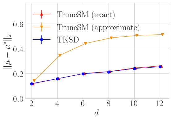
This plot shows mean estimation error over 64 trials in a simple task of estimating the mean of Gaussian distribution truncated within a \(\ell_2\) ball, whilst varying the dimension \(d\). We compare TKSD to TruncSM under two scenarios, the exact scenario is where TruncSM has access to the explicit boundary formulation, and the approximate scenario is where it only has access to a finite number of samples on the boundary - the same samples we give to TKSD. Overall, TKSD trades blows with TruncSM (exact), and does significantly better than TruncSM (approximate), even though it is given the exact same information. So with less information, TKSD still matches the state-of-the-art method.

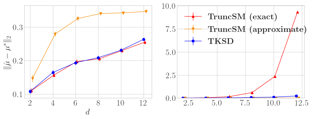
This second plot shows the same experiment setup but for truncation of the \(\ell_1\) ball instead of the \(\ell_2\) ball. We also plot runtime for all methods. Similar to the last experiment, TKSD and TruncSM (exact) have comparable errors across all dimensions. The main message in this example is how long it takes TruncSM (exact) to run, because analytically calculating the functional boundary for high dimension \(\ell_1\) balls is costly, combinatorically costly with \(d\), in fact. TruncSM (approximate) is, like before, not very good, even though it is cheaper to run. Both instances of TruncSM have issues, whereas TKSD seems to be the superior option.

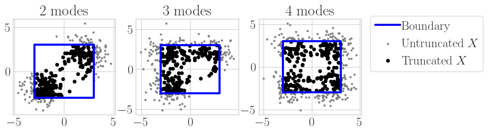
The next set of experiments contains a more complex setup, which is estimating multiple modes of a mixed Gaussian distribution. This is a similar experiment setup to before, except we are estimating 2, 3 and 4 means of a Gaussian at the same time. Figure 3 shows the experiment visually; as we vary the number of mixture modes, the distribution becomes more complex and thus harder to estimate accurately.

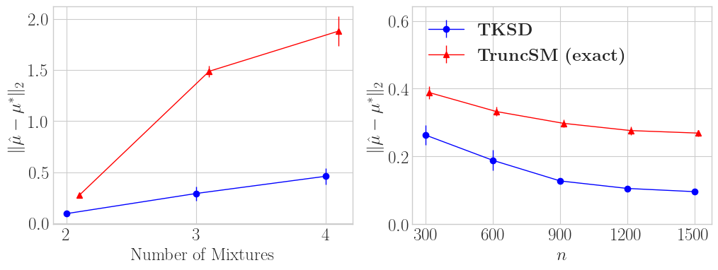
Figure 4 shows the mean estimation error across 64 trials for TKSD and TruncSM (exact). We vary the number of mixture modes (left) from 2-4, and measure how that changes the error across both methods. We also fix the number of mixture modes as 2, and vary sample size \(n\) (right), and also compare the error. Across both experiments, TKSD is Ivan Drago, and TruncSM is Apollo Creed (sorry). TKSD has a significantly smaller error than TruncSM.

Regression Example

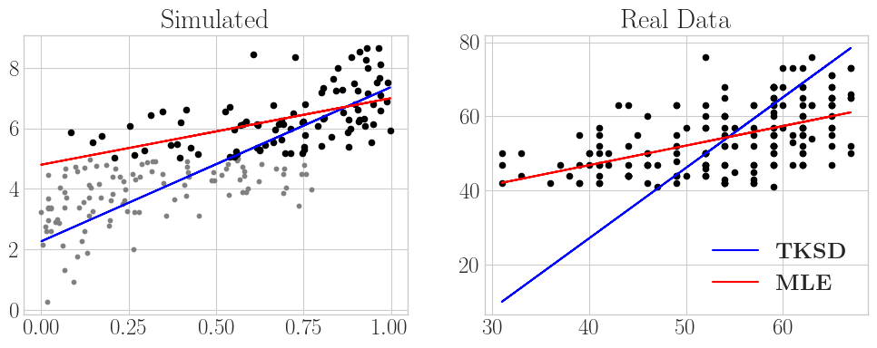
Let’s look at one specific example before we go, a simple linear regression. Since TKSD is a density estimation method, we can use it to estimate parameters of the (conditional) mean of a Normal distribution, given some feature variables. Truncation happens in the \(y\) domain, so that all of our data is truncated according to conditions on \(y\). In the first plot, we simulate a regression setting where we know the true parameters and can see the untruncated data. We pretend to only observe \(y_i \geq 5\), \(\forall i = 1,\dots, n\), and fit the model to the remaining data. When comparing the TKSD fit to a naive least squares implementation (MLE) which does not account for truncation, you can clearly see the difference that accounting for this simple truncation makes in our regression line.

The second plot is an experiment on a real-world dataset, given by UCLA: Statistical Consulting Group [5]. This dataset contains student test scores in a school for which the acceptance threshold is 40/100, and therefore the response variable (the test scores) are truncated below by 40 and above by 100. Since no scores get close to 100, we only consider one-sided truncation at \(y = 40\). The aim of the regression is to model the response variable, the test scores, based on a single covariate of each students’ corresponding score on a different test. We see very clearly in this example that accounting for this truncation seems to give a better fit than a regular least squares solution.

References

[1] Liu, S., Kanamori, T., and Williams, D. J. Estimating density models with truncation boundaries using score matching. Journal of Machine Learning Research, 23(186):1–38, 2022.
[2] Hyvärinen, A. Estimation of non-normalized statistical models by score matching. Journal of Machine Learning Research, 6(24):695–709, 2005.
[3] Barp, A., Briol, F.-X., Duncan, A., Girolami, M., and Mackey, L. Minimum stein discrepancy estimators. In Advances in Neural Information Processing Systems, volume 32, 2019.
[4] Chwialkowski, K., Strathmann, H., and Gretton, A. A kernel test of goodness of fit. In Proceedings of The 33rd International Conference on Machine Learning, volume 48 of Proceedings of Machine Learning Research, pp. 2606–2615. PMLR, 2016
[5] UCLA: Statistical Consulting Group. Truncated regression — stata data analysis examples. URL https://stats.oarc.ucla.edu/stata/dae/truncated-regression/. Accessed March 17, 2023.
Daniel Williams
CDT Student
I have a PhD in statistics/machine learning/data science/AI (whatever you would like to call it) from the University of Bristol, under the COMPASS CDT. I previously studied a masters in mathematics at the University of Exeter. My research was primarily on truncated density estimation and unnormalised models. But I am also interested in AI more generally, including all the learnings, Machine, Deep and Reinforcement (as well as some others!).